
这组文章整理自 2024 年的课程学习笔记,保留原练习、代码和图表。运行前请先看系列目录中的环境与数据说明。 查看系列目录。
Graph-based learning
(This notebook is partly based on a workshop by Robert Peach and Mauricio Barahona: https://github.com/peach-lucien/networks_workshop/tree/main)
Here, we will go through an analysis of the Caenorhabditis elegans (C. elgans) connectome. C. elegans is the only organism for which the wiring diagram of its complete nervous system has been mapped with reasonable accuracy at the cellular level. Despite this structural information, which has been available for decades, it still proves difficult to understand the system, e.g, resolving the functional involvement of specific neurons in defined behavioural responses.
We will use data that Robert Peach has reconstructed from the following article with the inclusion of muscles https://www.nature.com/articles/nature24056. The connectome is composed of directed connections from one neuron to another neuron in accordance with their biological influence.
Each node falls into one of four categories:
- Sensory neurons (S)
- Inter neurons (I)
- Motor neurons (M)
- Muscles (U)
Therefore, we can model the nematode nervous system as a directed network whose nodes include neurons and muscles, and whose links represent the electrical and chemical synaptic connections between them, including neuromuscular junctions. The weights of the edges correspond to the number of synaptic connections between a pair of neurons.
1 | import matplotlib |
Pre-processing C. Elegans network data
We are provided with an adjacency matrix A raw A_\text{raw} Araw of the C. Elgans network and metadata for the nodes (including neuron type, name and neuron class).
1 | import pandas as pd |
1 | <input type="file" id="files-563ef582-60ea-4369-bc5e-538e50630b68" name="files[]" multiple disabled |
//
// Licensed under the Apache License, Version 2.0 (the “License”);
// you may not use this file except in compliance with the License.
// You may obtain a copy of the License at
//
// http://www.apache.org/licenses/LICENSE-2.0
//
// Unless required by applicable law or agreed to in writing, software
// distributed under the License is distributed on an “AS IS” BASIS,
// WITHOUT WARRANTIES OR CONDITIONS OF ANY KIND, either express or implied.
// See the License for the specific language governing permissions and
// limitations under the License.
/**
- @fileoverview Helpers for google.colab Python module.
*/
(function(scope) {
function span(text, styleAttributes = {}) {
const element = document.createElement(‘span’);
element.textContent = text;
for (const key of Object.keys(styleAttributes)) {
element.style[key] = styleAttributes[key];
}
return element;
}
// Max number of bytes which will be uploaded at a time.
const MAX_PAYLOAD_SIZE = 100 * 1024;
function _uploadFiles(inputId, outputId) {
const steps = uploadFilesStep(inputId, outputId);
const outputElement = document.getElementById(outputId);
// Cache steps on the outputElement to make it available for the next call
// to uploadFilesContinue from Python.
outputElement.steps = steps;
return _uploadFilesContinue(outputId);
}
// This is roughly an async generator (not supported in the browser yet),
// where there are multiple asynchronous steps and the Python side is going
// to poll for completion of each step.
// This uses a Promise to block the python side on completion of each step,
// then passes the result of the previous step as the input to the next step.
function _uploadFilesContinue(outputId) {
const outputElement = document.getElementById(outputId);
const steps = outputElement.steps;
const next = steps.next(outputElement.lastPromiseValue);
return Promise.resolve(next.value.promise).then((value) => {
// Cache the last promise value to make it available to the next
// step of the generator.
outputElement.lastPromiseValue = value;
return next.value.response;
});
}
/**
- Generator function which is called between each async step of the upload
- process.
- @param {string} inputId Element ID of the input file picker element.
- @param {string} outputId Element ID of the output display.
- @return {!Iterable<!Object>} Iterable of next steps.
/
function uploadFilesStep(inputId, outputId) {
const inputElement = document.getElementById(inputId);
inputElement.disabled = false;
const outputElement = document.getElementById(outputId);
outputElement.innerHTML = ‘’;
const pickedPromise = new Promise((resolve) => {
inputElement.addEventListener(‘change’, (e) => {
resolve(e.target.files);
});
});
const cancel = document.createElement(‘button’);
inputElement.parentElement.appendChild(cancel);
cancel.textContent = ‘Cancel upload’;
const cancelPromise = new Promise((resolve) => {
cancel.onclick = () => {
resolve(null);
};
});
// Wait for the user to pick the files.
const files = yield {
promise: Promise.race([pickedPromise, cancelPromise]),
response: {
action: ‘starting’,
}
};
cancel.remove();
// Disable the input element since further picks are not allowed.
inputElement.disabled = true;
if (!files) {
return {
response: {
action: ‘complete’,
}
};
}
for (const file of files) {
const li = document.createElement(‘li’);
li.append(span(file.name, {fontWeight: ‘bold’}));
li.append(span((${file.type || 'n/a'}) - ${file.size} bytes, +last modified: ${ file.lastModifiedDate ? file.lastModifiedDate.toLocaleDateString() : 'n/a'} - ));
const percent = span(‘0% done’);
li.appendChild(percent);
1 | outputElement.appendChild(li); |
}
// All done.
yield {
response: {
action: ‘complete’,
}
};
}
scope.google = scope.google || {};
scope.google.colab = scope.google.colab || {};
scope.google.colab._files = {
_uploadFiles,
_uploadFilesContinue,
};
})(self);
1 | Saving celegans_adjacency_transposed.csv to celegans_adjacency_transposed.csv |
We can first plot A raw A_\text{raw} Araw as a heatmap and observe that the matrix is very sparse with values ranging from 0 to over 30.
1 | fig, ax = plt.subplots(1) |
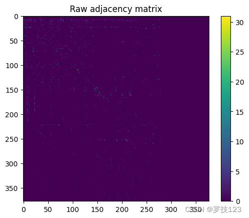
Arguably, this visualisation of the adjacency matrix is not very illuminating. We will discuss better ways to visualise our data below. Let’s first review the node metadata.
1 | # look up node data |
| type | name | neuron_class | |
|---|---|---|---|
| 0 | I | ADAR | ADA |
| 1 | I | ADAL | ADA |
| 2 | S | ADFL | ADF |
| 3 | S | ASHL | ASH |
| 4 | I | AVDR | AVD |
1 | </button> |
1 | <script> |
<svg xmlns=“http://www.w3.org/2000/svg” height=”24px”viewBox=“0 0 24 24”
width=“24px”>
We encode the node types with numerical values.
1 | # transform node type into integers |
Let us check some basic properties of the graph, in particular whether is undirected and unweighted.
1 | # check properties of graph |
1 | Graph is undirected: False |
To simply our analysis below, we go from the raw adjacency matrix A raw A_\text{raw} Araw to the adjacency matrix A A A of an undirected and unweighted graph, where A i j = A j i = 1 A_{ij}=A_{ji}=1 Aij=Aji=1 if either A raw , i j > 0 A_{\text{raw}, ij}>0 Araw,ij>0 or A raw , j i > 0 A_{\text{raw}, ji}>0 Araw,ji>0 and A i j = A j i = 0 A_{ij}=A_{ji}=0 Aij=Aji=0 otherwise.
1 | ## EDIT THIS CELL |
1 | # double check if graph is now undirected and unweighted |
1 | Graph is undirected: True |
Degree distribution of undirected C. Elegans network
Let us now compute the number of nodes and eges of our undirected unweighted graph given by A A A.
1 | ## EDIT THIS CELL |
1 | Number of nodes: 377 |
As a first step of our analysis we look at the degree distribution d = A 1 \boldsymbol{d}=A\boldsymbol{1} d=A1.
1 | ## EDIT THIS CELL |
1 | # visualise degree distributions |
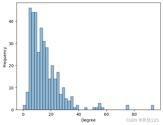
Let us look up the names and types two highest degree nodes.
1 | ## EDIT THIS CELL |
1 | Highest degree neuron is AVAR of type I. |
We notice that the two highest degree nodes are both of the same type inter neuron type (I). This suggests that it will be instructive to plot the degree distribution for the four different types of nodes.
1 | # visualise degree distributions for the four different types |
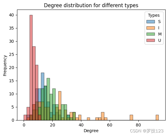
From the degree distrubtions we can observe that the inter neurons (I) seem to have a higher degree, i.e., they are most connected, and the muscles (U) are the least connected in the nervous system.
We will define node colours consistent with this plot to use for later.
1 | # we define node colours consistent with the plot above |
Spectral analysis of symmetric normalised Laplacian
We focus our analysis on the spectrum of the normalised graph Laplacian L sym L_\text{sym} Lsym, which is given by:
L sym = D − 1 / 2 L D − 1 / 2 , L_\text{sym}=D^{-1/2} L D^{-1/2}, Lsym=D−1/2LD−1/2,where L = D − A L=D-A L=D−A is the combinatorial Laplacian and D D D the diagonal degree matrix.
1 | ## EDIT THIS CELL |
We are now interested in the spectral decomposition of L sym L_\text{sym} Lsym. We know that the first (smallest) eigenvalue is λ 1 = 0 \lambda_1=0 λ1=0 with corresponding eigenvector v 1 = D 1 / 2 1 \boldsymbol{v}_1=D^{1/2}\boldsymbol{1} v1=D1/21 (can you prove this?).
1 | # the square-root of the degree vector is the zero eigenvector to eigenvalue 0 |
1 | True |
To compute the full spectrum of L sym L_\text{sym} Lsym, we use the fact that it is a real symmetric matrix and sort the eigenvalues (and corresponding eigenvectors) in ascending order.
1 | ## EDIT THIS CELL |
We can visualise the spectrum of L sym L_\text{sym} Lsym.
1 | # plot eigenvalues |
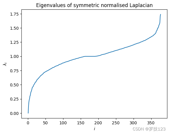
We confirm that the first eigenvalue is λ 1 = 0 \lambda_1=0 λ1=0, but we are more interested in the second eigenvalue λ 2 > 0 \lambda_2>0 λ2>0, which is also called the algebraic connectivity.
1 | ## EDIT THIS CELL |
1 | First eigenvalue: -0.0 |
As λ 2 \lambda_2 λ2, is small we expect that the graph has a good bipartition. We will study this later.
Graph visualisation using Laplacian eigenmaps
But first we will use the second (Fiedler) eigenvector v 2 \boldsymbol{v}_2 v2 and third eigengenvector v 3 \boldsymbol{v}_3 v3 to visualise the network. Using these two Laplacian eigenvectors (also called Laplacian eigenmaps) as x \boldsymbol{x} x and y \boldsymbol{y} y coordinates of the nodes gives us a good two-dimensional representation of the graph (a spectral embedding). We can improve the visualisation when normalising the coordinates such that x = D − 1 / 2 v 2 \boldsymbol{x}=D^{-1/2}\boldsymbol{v}_2 x=D−1/2v2 and y = D − 1 / 2 v 3 \boldsymbol{y}=D^{-1/2}\boldsymbol{v}_3 y=D−1/2v3.
1 | ## EDIT THIS CELL |
We can simply plot the graph by drawing lines between the embeddings of two connected nodes. Additionally, we can scale the node size dependent on the degree.
1 | # plot |
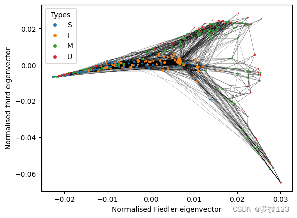
We observe that the muscles (U) are located in the periphery of the network, while the most connected inter neurons (I) are located in the center.
Another way to visualise the graph is to directly use the node degree d \boldsymbol{d} d as the y-coordinate, i.e., y = d \boldsymbol{y}=\boldsymbol{d} y=d.
1 | # plot |
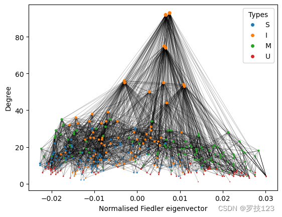
This visualisation gives a more decluttered picture and is very useful to distinguish the different node types in the network. For the rest of the notebook, we will thus use this visualisation.
As you have learnt by now, graph visualisation is a very interesting topic in itself and there are many algorithms to plot various graphs, including very large ones.
Questions:
- Why is graph visualisation not unique?
- Can you come up with alternative graph visualisations?
Bipartitioning using Fiedler eigenvector
We will now use the second (Fiedler) eigenvector v 2 \boldsymbol{v}_2 v2 to bipartition the network into two communities, given by the sign of v 2 \boldsymbol{v}_2 v2.
1 | ## EDIT THIS CELL |
As the algebraic connectivity λ 2 \lambda_2 λ2 is small, we expect that the bipartition is very balanced. To confirm this we compute the number of nodes and the total degree of both communities.
1 | ## EDIT THIS CELL |
1 | Size of first community: 181 |
Indeed, we find that the communities of the bipartition contain a very similar number of nodes and also have a similar total degree. It is illustrative to visualise the bipartition in the network.
1 | # use different colours for bipartition |
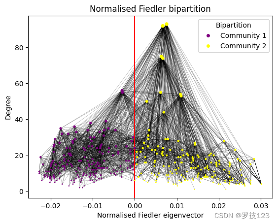
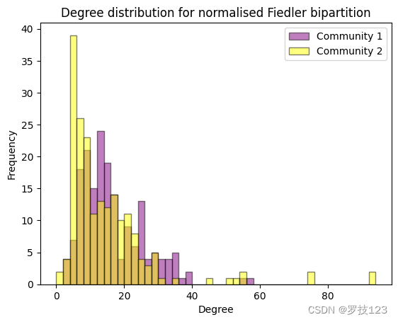
While the nodes with the highest degree belong to community 2, the degree distribution seems to be quite uniform between the two communities. We confirm this by plotting the degree distributions as histograms.
1 | # visualise degree distributions for both communities |
Spectral clustering using more Laplacian eigenvectors
To go beyond bipartitions, we can use more Laplacian eigenvectors and apply what is called spectral clustering, where we apply k k k-means clustering to the Laplacian eigenmaps (see Section 12.4.2.1 in the lecture notes).
Code for k-means clustering from Week 7
To use k k k-means clustering we first copy-paste the code from Week 7.
1 | def compute_within_distance(centroids, X, labels): |
Using k-means for spectral clustering
Let us define a N × r N\times r N×r feature matrix X X X that contains the first r > 0 r>0 r>0 Laplacian eigenvectors (corresponding to non-zero eigenvalues) as columns. For spectral clustering, it is recommended to first obtain a normalised feature matrix Y Y Y from X X X following the famous paper by Ng, Jordan, and Weiss 2001:
Y i j = X i j ∑ j = 1 r X i j 2 , Y_{ij}=\frac{X_{ij}}{\sqrt{\sum_{j=1}^r X_{ij}^2}}, Yij=∑j=1rXij2Xij,such that the rows of Y Y Y have unit lengths. We compute Y Y Y for r = 10 r=10 r=10.
1 | ## EDIT THIS CELL |
Treating each row of Y Y Y as a point in R r \mathbb{R}^r Rr gives us r r r-dimensional embeddings for the nodes in the network. We can then cluster the network using k k k-means. Our question is whether we can retrieve the four node types using spectral clustering, so we set k = 4 k=4 k=4.
1 | ## EDIT THIS CELL |
Already through visualising the partition, it seems like there is a low correspondence to the node types when compared to the visualsiations above.
1 | # use different colours for spectral partition |
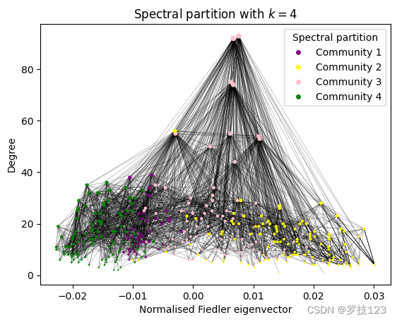
We also observe that the degree distributions of the different clusters in the spectral partition are very similar, so unlike the degree distributions according to the different node types discussed above.
1 | # visualise degree distributions for the four spectral communities |
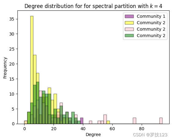
However, it is expected that the spectral partition is not consistent with the partition of node types because it actually reflects the physical positions of the neurons in the organism (we can’t show this here). This is the case because the spectral partition is obtained from the Laplacian that encodes the connectivity of neurons in a physical organism.
Using Normalised Variation of Information for comparing partitions
We implement the Normalised Variation of Information (NVI) to compare the spectral partition with the node types (which constitutes an alternative partition of the network), see Section 10.7 in the updated lecture notes. For two partitions P 1 \mathcal{P}_1 P1 and P 2 \mathcal{P}_2 P2 you can compute the entropies E ( P 1 ) E(\mathcal{P}_1) E(P1) and E ( P 2 ) E(\mathcal{P}_2) E(P2) and the mutual information M I ( P 1 , P 2 ) MI(\mathcal{P}_1,\mathcal{P}_2) MI(P1,P2). The NVI is then given by:
N V I ( P 1 , P 2 ) = E ( P 1 ) + E ( P 2 ) − 2 M I ( P 1 , P 2 ) E ( P 1 ) + E ( P 2 ) − M I ( P 1 , P 2 ) NVI(\mathcal{P}_1,\mathcal{P}_2)=\frac{ E(\mathcal{P}_1)+E(\mathcal{P}_2)-2 MI(\mathcal{P}_1,\mathcal{P}_2)}{E(\mathcal{P}_1)+E(\mathcal{P}_2)- MI(\mathcal{P}_1,\mathcal{P}_2)} NVI(P1,P2)=E(P1)+E(P2)−MI(P1,P2)E(P1)+E(P2)−2MI(P1,P2)The NVI is a metric on the space of partitions and ranges between 0 (partitions are the same) to 1.
1 | ## EDIT THIS CELL |
You can check your implementation with the following cell.
1 | # check for two test cases |
We can now compute the NVI between the spectral partition and the node type.
1 | ## EDIT THIS CELL |
1 | NVI of spectral partition and node types: 0.837 |
The NVI confirms our observations that the spectral partition is actually not very similar to the partition of node types.
We conclude here by double-checking some of the metric properties of the NVI.
1 | # we can check that the NVI is symmetric |
Analysing the directed C. Elegans network
As the node types I, S, M and U actually correspond to different functionalities of neurons in the organism, we expect that they play different “roles” in the network. We saw this already when looking at the degree distribution of the different types, where the inter neurons (I) had the the highest degrees.
We can improve our analysis by looking not only at the degree in the undirected network, but studing the in- and out-degrees in the directed C. Elegans network.
Let us start with compiling the directed unweighted C. Elegans network whose adjacency matrix we denote by B B B such that B i j = 1 B_{ij}=1 Bij=1 if A raw , i j > 0 A_{\text{raw}, ij}>0 Araw,ij>0 and B i j = 0 B_{ij}=0 Bij=0 otherwise.
1 | ## EDIT THIS CELL |
We can then compute the in- and out-degrees of B B B.
1 | ## EDIT THIS CELL |
We now plot the neurons in a scatter plot with x-coordinate given by the in-degree and y-coordinate given by the out-degree.
1 | # scatter plot in- and out-degrees |
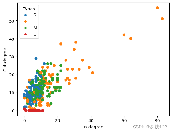
We can see that the combination of in- and out-degreens helps us to distinguish the different types. Most strikingly, the muscles have a very low out-degree (mostly 0) and only incoming nodes as they sit at the bottom of the hierarchy in the nervous system of C. Elegans.
Although it doesn’t look very promising, we will apply k-means clustering to a feature matix Z Z Z that has the in- and out-degrees as columns.
1 | ## EDIT THIS CELL |
1 | <ipython-input-27-8846dba3c782>:57: RuntimeWarning: Mean of empty slice. |
We can visualise the obtained clustering in a scatter plot.
1 | # scatter plot in- and out-degrees |
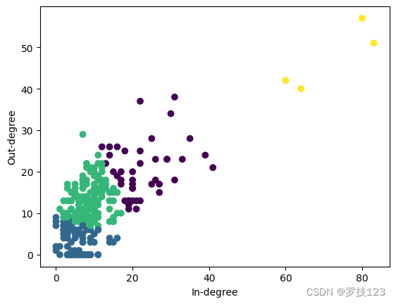
To quantify the correspondence to the ground truth node types, we evaluate the NVI of the “in-degree out-degree partition” and the node types and observe a slightly lower value as compared to spectral clustering.
1 | ## EDIT THIS CELL |
1 | NVI of in-degree out-degree partition and node types: 0.826 |
The analysis of in-degree and out-degree patterns of nodes aims at recovering different roles in the network. If you want to read more on how to distinguish nodes in a graph based on in-coming and out-going paths you can have a look at a paper by Kathryn Cooper and Mauricio Barahona on Role-based similarity in directed networks: https://arxiv.org/abs/1012.2726
 微信
微信 支付宝
支付宝