一起学习机器学习（12）：高斯混合模型

这组文章整理自 2024 年的课程学习笔记，保留原练习、代码和图表。运行前请先看系列目录中的环境与数据说明。 查看系列目录。

Clustering using Gaussian Mixture Models

In this notebook, we will learn about mixture models that find applications in clustering. To start with, we will focus on two clusters and we will use the expectation-maximisation algorithm for optimisation.

1
2
3
4
5
6

# import libraries
import numpy as np
import numpy.testing as npt
import pandas as pd
import matplotlib.pyplot as plt
from scipy.stats import multivariate_normal

Section 1: Gaussian Mixture Model

Following the lecture notes, the Gaussian Mixture Model (GMM) is given by:
$$P(\mathbf{X}=\mathbf{x})=\sum _{k=1}^K{\pi }_k{p}_k(\mathbf{x}|\mathbf{\theta }).$$
Here $K$ is the number of clusters described as mixture components, each of which are multivariate normal distributions:
$$p_k(\mathbf{x}|\mathbf{\theta })=(2\pi {)}^{-k/2}\det ({\mathbf{\Sigma }}_k{)}^{-1/2}\exp \left(-\frac{1}{2}(\mathbf{x}-{\mathbf{\mu }}_k{)}^{\mathsf{T}}{{\mathbf{\Sigma }}_k}^{-1}(\mathbf{x}-{\mathbf{\mu }}_k)\right),$$
where $\mathbf{\theta }=\{{\pi }_k,{\mu }_k,{\Sigma }_k{\}}_{k=1,2,...,K}$ is the vector of parameters consiting of the mixture weights ${\pi }_k$, mixture component means ${\mathbf{\mu }}_k$ and mixture component covariance matrices ${\mathbf{\mu }}_k$.

We start by implementing a class for the GMM model.

1
2
3
4
5
6
7
8
9
10
11
12
13
14
15
16
17
18
19
20
21
22
23
24
25
26
27
28
29
30
31
32
33
34
35
36

import copy

class GMModel:
    """Struct to define Gaussian Mixture Model.
        Attributes:
            X (np.ndarray): the samples array, shape (N, p).
            k (int): number of mixture components, i.e. number of clusters.
            weights (np.ndarray): mixture weights.
            mu (np.ndarray): mixture component means for each cluster.
            sigma (np.ndarray): mixture component covariance matrix for each cluster
    """

    def __init__(self, X, k):
        """Initialises parameters through random split of the data"""

        self.k = k

        # initial weights given to each cluster are stored in pi or P(Ci=j)
        self.pi = np.full(shape=self.k, fill_value=1/self.k)

        # initial weights given to each data point wrt to each cluster or P(Xi|Ci=j)
        self.weights = np.full(shape=X.shape, fill_value=1/self.k)

        n, m = X.shape
        # dataset is divided randomly into k parts of unequal sizes
        random_row = np.random.randint(low=0, high=n, size=self.k)

        # initial value of mean of k Gaussians
        self.mu = [ X[row_index,:] for row_index in random_row ]

        # initial value of covariance matrix of k Gaussians
        self.sigma = [np.cov(X.T) for _ in range(self.k) ]

    def copy(self):
        """Return an isolated copy."""
        return copy.deepcopy(self)

We can perform ‘soft’ clustering of the data using the cluster probabilities of the data:
$$r_{ik}(\mathbf{\theta })=P(Z=k|\mathbf{X}={\mathbf{x}}_i,\mathbf{\theta })=\frac{{\pi }_k{p}_k({\mathbf{x}}_i|\mathbf{\theta })}{{\sum }_{k^{\prime }=1}^K{\pi }_{k^{\prime }}{p}_{k^{\prime }}({\mathbf{x}}_i|\mathbf{\theta })}$$
This denotes the probability of data point $i$ to belong to cluster $k$. Generally, this yields a distribution over each data point.

1
2
3
4
5
6
7
8
9
10
11
12
13
14
15
16
17
18
19
20
21
22
23
24
25
26
27

## EDIT THIS FUNCTION
def cluster_probabilities(gmm, X):
    """
    Predicts probability of each data point with respect to each cluster

    Args:
        gmm (GMModel): the GMM model.
        X (np.ndarray): the samples array, shape: (N, p).

    Returns:
        (np.ndarray): weights of each data point w.r.t each cluster, shape (N, k)
    """

    # n has the number of rows while p has the number of columns of dataset X
    n, p = X.shape
    # Creates a n*k matrix denoting likelihood belonging to each cluster
    likelihood = np.zeros((n, gmm.k))
    for i in range(gmm.k):
        # likelihood of data belonging to i-th cluster
        distribution = multivariate_normal(mean=gmm.mu[i],
                                           cov=gmm.sigma[i])
        likelihood[:,i] = distribution.pdf(X)

    numerator = likelihood * gmm.pi # <-- SOLUTION
    denominator = numerator.sum(axis=1, keepdims=True) # <-- SOLUTION
    weights = numerator / denominator
    return weights

Let’s make sure that we pass the following test cases.

1
2
3
4
5
6
7
8
9
10

np.random.seed(2)
X_testing = np.array([[1.0, 2.0],
                      [3.0, -1.0],
                      [-3.0, 1.0]])
expected_output = np.array([[0.88079708, 0.11920292],
                            [0.11920292, 0.88079708],
                            [0.5       , 0.5       ]])

gmm_test = GMModel(X_testing, 2)
npt.assert_allclose(cluster_probabilities(gmm_test, X_testing), expected_output)

For visualisation it is useful to present the results as hard clusters on the output through the argmax of the cluster distribution:

1
2
3
4
5

## EDIT THIS FUNCTION
def predict(gmm, X):
    """Performs hard clustering."""
    weights = cluster_probabilities(gmm,X)
    return np.argmax(weights, axis=1) # <-- SOLUTION

Let us initially try GMM clustering on synthetic data. Sampling Gaussian mixtures is relatively straightforward.

1
2
3
4
5
6
7
8
9
10

np.random.seed(42)
def testdata():
    cov = np.array([[6, -3], [-3, 3.5]])
    A = np.random.multivariate_normal([0, 0], cov, size=50)
    B = np.random.multivariate_normal([10, 5], cov, size=50)
    return np.vstack((A,B)) # combine

data0=testdata()
plt.scatter(data0[:,0],data0[:,1])
plt.show()

​

​

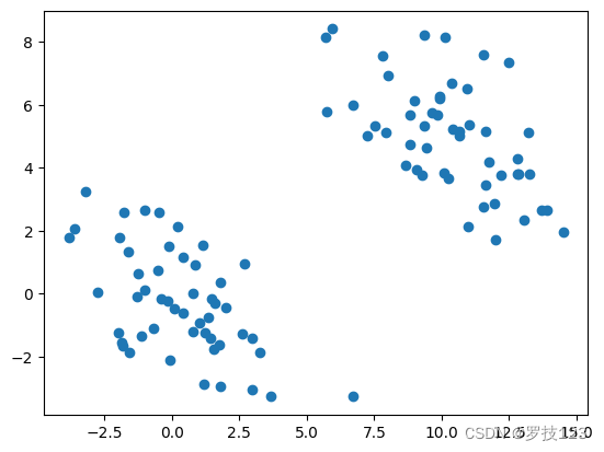
We borrow some plot functions from the Python Data Science Handbook to visualise the mixture model.

See https://jakevdp.github.io/PythonDataScienceHandbook/05.12-gaussian-mixtures.html

1
2
3
4
5
6
7
8
9
10
11
12
13
14
15
16
17
18
19
20
21
22
23
24
25
26
27
28
29
30
31
32
33
34

from matplotlib.patches import Ellipse
import matplotlib.pyplot as plt

def draw_ellipse(position, covariance, ax=None, **kwargs):
    """Draw an ellipse with a given position and covariance"""
    ax = ax or plt.gca()

    # Convert covariance to principal axes
    if covariance.shape == (2, 2):
        U, s, Vt = np.linalg.svd(covariance)
        angle = np.degrees(np.arctan2(U[1, 0], U[0, 0]))
        width, height = 2 * np.sqrt(s)
    else:
        angle = 0
        width, height = 2 * np.sqrt(covariance)

    # Draw the Ellipse
    for nsig in range(1, 4):
        ax.add_patch(Ellipse(position, nsig * width, nsig * height,
                             angle, **kwargs))

def gmm_plot(gmm, X, label=True, ax=None):
    ax = ax or plt.gca()
    labels = predict(gmm, X)
    if label:
        ax.scatter(X[:, 0], X[:, 1], c=labels, s=40, cmap='viridis', zorder=2)
    else:
        ax.scatter(X[:, 0], X[:, 1], s=40, zorder=2)
    ax.axis('equal')

    w_factor = 0.2 / gmm.weights.max()
    for pos, covar, w in zip(gmm.mu, gmm.sigma, gmm.pi):
        draw_ellipse(pos, covar, alpha=w * w_factor)
    return ax

We can now cluster the synthetic data using a GMM model with randomly initialised parameters:

1
2
3

np.random.seed(4)
gmm = GMModel(data0,2)
gmm_plot(gmm, data0)

1
2
3
4
5
6
7
8

<ipython-input-7-0ad8cdc6bec6>:19: MatplotlibDeprecationWarning: Passing the angle parameter of __init__() positionally is deprecated since Matplotlib 3.6; the parameter will become keyword-only two minor releases later.
  ax.add_patch(Ellipse(position, nsig * width, nsig * height,





<Axes: >

​

​

As expected, the two clusters obtained from the randomly initialised GMM do not match the ground truth clusters at all because we first need to learn the parameters.

Section 2: Fitting Gaussian Mixture Models using the EM algorithm

We employ the EM algorithm to fit the data. The algorithm iteratively updates parameters of the Gausian Mixture. The algorithm is guaranteed to improve (or at least not worsen) the marginal likelihood of the data. The algorithm updates the mixture weights:
$${\pi }_k^{(n+1)}=\frac{1}{N}\sum _{i=1}^N{r}_{ik}({\mathbf{\theta }}^{(n)}),$$
and computes the cluster means using a weighted mean:
$${\mathbf{\mu }}_k^{(n+1)}=\sum _{i=1}^N{w}_{ik}({\mathbf{\theta }}^{(n)}){\mathbf{x}}_i$$
and similarly for the covariances according to
$${\mathbf{\Sigma }}_k^{(n+1)}=\sum _{i=1}^N{w}_{ik}({\mathbf{\theta }}^{(n)})({\mathbf{x}}_i-{\mathbf{\mu }}_k)({\mathbf{x}}_i-{\mathbf{\mu }}_k{)}^T.$$
The weights are obtained from the cluster probabilities via
$$w_{ik}({\mathbf{\theta }}^{(n)})=\frac{r_{ik}({\mathbf{\theta }}^{(n)})}{{\sum }_{i^{\prime }}{r}_{i^{\prime }k}({\mathbf{\theta }}^{(n)})}$$
A single step of this iteration is implemented in the following function:

1
2
3
4
5
6
7
8
9
10
11
12
13
14
15
16
17
18
19
20
21
22
23
24
25
26
27
28
29

## EDIT THIS FUNCTION
def gmm_fit_step(gmm, X):
    """
    Performs an EM step by updating all parameters.

    Args:
        gmm (GMModel): the current GMM model.
        X (np.ndarray): the samples array, shape: (N, p).

    Returns:
        gmm (GMModle): an updated GMM model after applying the E-M steps.
    """
    gmm = gmm.copy()

    # E-Step: update weights and pi holding mu and sigma constant
    weights = cluster_probabilities(gmm, X) # <-- SOLUTION
    gmm.pi = weights.mean(axis=0) # <-- SOLUTION

    # M-Step: update mu and sigma holding pi and weights constant
    for i in range(gmm.k):
        weight = weights[:, [i]]
        total_weight = weight.sum()

        gmm.mu[i] = (X * weight).sum(axis=0) / total_weight # <-- SOLUTION
        gmm.sigma[i] = np.cov((X-gmm.mu[i]).T,
                              aweights=(weight/total_weight).flatten(),
                              bias=True) # <-- SOLUTION (check np.cov documentation for weighted computation)

    return gmm

Let’s make sure we pass the following test case.

1
2
3
4
5
6
7
8
9
10
11
12
13

np.random.seed(2)
X_testing = np.array([[1.0, 2.0],
                      [3.0, -1.0],
                      [-3.0, 1.0]])

gmm_test = GMModel(X_testing, 2)
gmm_test = gmm_fit_step(gmm_test, X_testing)
npt.assert_allclose(gmm_test.mu[0], np.array([-0.1743961 ,  1.42826082]))
npt.assert_allclose(gmm_test.mu[1], np.array([0.84106277, -0.09492749]))
npt.assert_allclose(gmm_test.sigma[0], np.array([[4.27200158, 0.18507338],
                                                [0.18507338, 0.72166518]]))
npt.assert_allclose(gmm_test.sigma[1], np.array([[ 7.6568645 , -2.52281695],
                                                [-2.52281695,  1.22939462]]))

One EM iteration does not significantly improve the result:

1
2

gmm_fit_step(gmm,data0)
gmm_plot(gmm,data0)

1
2
3
4
5
6
7
8

<ipython-input-7-0ad8cdc6bec6>:19: MatplotlibDeprecationWarning: Passing the angle parameter of __init__() positionally is deprecated since Matplotlib 3.6; the parameter will become keyword-only two minor releases later.
  ax.add_patch(Ellipse(position, nsig * width, nsig * height,





<Axes: >

​

​

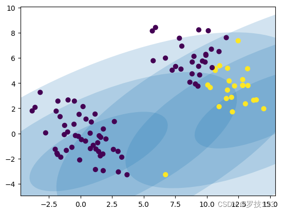
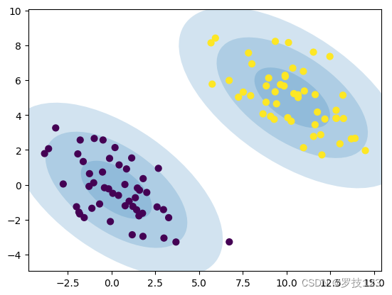
Let’s see if we can observe some improvement after several iterations:

1
2
3

for _ in range(10):
    gmm = gmm_fit_step(gmm,data0)
gmm_plot(gmm, data0)

1
2
3
4
5
6
7
8

<ipython-input-7-0ad8cdc6bec6>:19: MatplotlibDeprecationWarning: Passing the angle parameter of __init__() positionally is deprecated since Matplotlib 3.6; the parameter will become keyword-only two minor releases later.
  ax.add_patch(Ellipse(position, nsig * width, nsig * height,





<Axes: >

​

​

Section 3: Clustering of breast cancer data

In this final section we will again work with the Breast Cancer Wisconsin (Diagnostic) Data Set, which you first need to download and then load in this notebook. If you faced difficulties downloading this data set from Kaggle, you should download the file directly from Blackboard. The data set contains various aspects of cell nuclei of breast screening images of patients with (malignant) and without (benign) breast cancer. Our goal is to cluster the data without without the knowledge of the tumor being malignant or benign.

If you run this notebook locally on your machine, you will simply need to place the csv file in the same directory as this notebook.
If you run this notebook on Google Colab, you will need to use

from google.colab import files

upload = files.upload()

and then upload it from your local downloads directory.

1
2
3
4
5
6
7
8
9
10
11
12
13
14
15
16
17
18
19
20

from google.colab import files
upload = files.upload()
data = pd.read_csv('./data.csv')

# print shape and last 10 rows
print(data.shape)
data.tail(10)

# drop last column (extra column added by pandas)
data = data.drop(data.columns[-1], axis=1)
# set column id as dataframe index
data = data.set_index(data['id']).drop(data.columns[0], axis=1)

# convert categorical labels to numbers
diag_map = {'M': 1.0, 'B': -1.0}
data['diagnosis'] = data['diagnosis'].map(diag_map)

# split target from features
y = np.asarray(data.loc[:, 'diagnosis'])
X = np.asarray(data.iloc[:, 1:])

1
2
3
4
5
6
7

<input type="file" id="files-84fa5ae3-df7f-4d20-b21a-b3bde42dac5e" name="files[]" multiple disabled
   style="border:none" />
<output id="result-84fa5ae3-df7f-4d20-b21a-b3bde42dac5e">
 Upload widget is only available when the cell has been executed in the
 current browser session. Please rerun this cell to enable.
 </output>
 <script>// Copyright 2017 Google LLC

//
// Licensed under the Apache License, Version 2.0 (the “License”);
// you may not use this file except in compliance with the License.
// You may obtain a copy of the License at
//
// http://www.apache.org/licenses/LICENSE-2.0
//
// Unless required by applicable law or agreed to in writing, software
// distributed under the License is distributed on an “AS IS” BASIS,
// WITHOUT WARRANTIES OR CONDITIONS OF ANY KIND, either express or implied.
// See the License for the specific language governing permissions and
// limitations under the License.

/**

• @fileoverview Helpers for google.colab Python module.
  */
  (function(scope) {
  function span(text, styleAttributes = {}) {
  const element = document.createElement(‘span’);
  element.textContent = text;
  for (const key of Object.keys(styleAttributes)) {
  element.style[key] = styleAttributes[key];
  }
  return element;
  }

// Max number of bytes which will be uploaded at a time.
const MAX_PAYLOAD_SIZE = 100 * 1024;

function _uploadFiles(inputId, outputId) {
const steps = uploadFilesStep(inputId, outputId);
const outputElement = document.getElementById(outputId);
// Cache steps on the outputElement to make it available for the next call
// to uploadFilesContinue from Python.
outputElement.steps = steps;

return _uploadFilesContinue(outputId);
}

// This is roughly an async generator (not supported in the browser yet),
// where there are multiple asynchronous steps and the Python side is going
// to poll for completion of each step.
// This uses a Promise to block the python side on completion of each step,
// then passes the result of the previous step as the input to the next step.
function _uploadFilesContinue(outputId) {
const outputElement = document.getElementById(outputId);
const steps = outputElement.steps;

const next = steps.next(outputElement.lastPromiseValue);
return Promise.resolve(next.value.promise).then((value) => {
// Cache the last promise value to make it available to the next
// step of the generator.
outputElement.lastPromiseValue = value;
return next.value.response;
});
}

/**

• Generator function which is called between each async step of the upload
• process.
• @param {string} inputId Element ID of the input file picker element.
• @param {string} outputId Element ID of the output display.
• @return {!Iterable<!Object>} Iterable of next steps.
  /
  function uploadFilesStep(inputId, outputId) {
  const inputElement = document.getElementById(inputId);
  inputElement.disabled = false;

const outputElement = document.getElementById(outputId);
outputElement.innerHTML = ‘’;

const pickedPromise = new Promise((resolve) => {
inputElement.addEventListener(‘change’, (e) => {
resolve(e.target.files);
});
});

const cancel = document.createElement(‘button’);
inputElement.parentElement.appendChild(cancel);
cancel.textContent = ‘Cancel upload’;
const cancelPromise = new Promise((resolve) => {
cancel.onclick = () => {
resolve(null);
};
});

// Wait for the user to pick the files.
const files = yield {
promise: Promise.race([pickedPromise, cancelPromise]),
response: {
action: ‘starting’,
}
};

cancel.remove();

// Disable the input element since further picks are not allowed.
inputElement.disabled = true;

if (!files) {
return {
response: {
action: ‘complete’,
}
};
}

for (const file of files) {
const li = document.createElement(‘li’);
li.append(span(file.name, {fontWeight: ‘bold’}));
li.append(span(
(${file.type || 'n/a'}) - ${file.size} bytes, +
last modified: ${ file.lastModifiedDate ? file.lastModifiedDate.toLocaleDateString() : 'n/a'} - ));
const percent = span(‘0% done’);
li.appendChild(percent);

1
2
3
4
5
6
7
8
9
10
11
12
13
14
15
16
17
18
19
20
21
22
23
24
25
26
27
28
29
30
31
32
33
34
35
36
37
38
39

outputElement.appendChild(li);

const fileDataPromise = new Promise((resolve) => {
  const reader = new FileReader();
  reader.onload = (e) => {
    resolve(e.target.result);
  };
  reader.readAsArrayBuffer(file);
});
// Wait for the data to be ready.
let fileData = yield {
  promise: fileDataPromise,
  response: {
    action: 'continue',
  }
};

// Use a chunked sending to avoid message size limits. See b/62115660.
let position = 0;
do {
  const length = Math.min(fileData.byteLength - position, MAX_PAYLOAD_SIZE);
  const chunk = new Uint8Array(fileData, position, length);
  position += length;

  const base64 = btoa(String.fromCharCode.apply(null, chunk));
  yield {
    response: {
      action: 'append',
      file: file.name,
      data: base64,
    },
  };

  let percentDone = fileData.byteLength === 0 ?
      100 :
      Math.round((position / fileData.byteLength) * 100);
  percent.textContent = `${percentDone}% done`;

} while (position < fileData.byteLength);

}

// All done.
yield {
response: {
action: ‘complete’,
}
};
}

scope.google = scope.google || {};
scope.google.colab = scope.google.colab || {};
scope.google.colab._files = {
_uploadFiles,
_uploadFilesContinue,
};
})(self);

1
2

Saving data.csv to data.csv
(569, 33)

We start by visualising the ground-truth labels with respect to two featurs, the Mean Radius and Mean Texture of the tumor.

1
2
3
4
5
6
7
8
9

# plot for two features
labels = ["Malignant", "Benign"]
for i, c in enumerate(np.unique(y)):
    plt.scatter(X[:, 0][y==c],X[:, 1][y==c],label=labels[i]);
plt.xlabel("Mean Radius");
plt.ylabel("Mean Texture");
plt.title("Ground truth of Diagnoses");
plt.xlim([-5,40])
plt.legend();

​

​

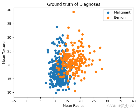
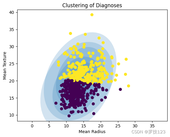
In the following, we apply GMM clustering to the data set only using these two features (Mean Radius and Mean Texture).

1
2
3
4
5
6
7
8
9
10
11
12

# restrict features
X = X[:,:2]

# initialise GMM model
np.random.seed(1)
gmm2 = GMModel(X,2)

# plot prediction
gmm_plot(gmm2,X)
plt.xlabel("Mean Radius");
plt.ylabel("Mean Texture");
plt.title("Clustering of Diagnoses");

1
2

<ipython-input-7-0ad8cdc6bec6>:19: MatplotlibDeprecationWarning: Passing the angle parameter of __init__() positionally is deprecated since Matplotlib 3.6; the parameter will become keyword-only two minor releases later.
  ax.add_patch(Ellipse(position, nsig * width, nsig * height,

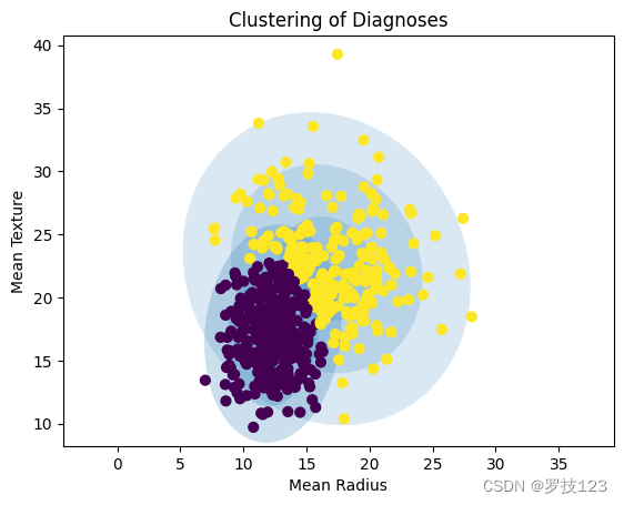
After initialising our GMM model we can fit it to the data.

1
2
3
4
5
6

for _ in range(100):
    gmm2 = gmm_fit_step(gmm2,X)
gmm_plot(gmm2,X)
plt.xlabel("Mean Radius");
plt.ylabel("Mean Texture");
plt.title("Clustering of Diagnoses");

1
2

<ipython-input-7-0ad8cdc6bec6>:19: MatplotlibDeprecationWarning: Passing the angle parameter of __init__() positionally is deprecated since Matplotlib 3.6; the parameter will become keyword-only two minor releases later.
  ax.add_patch(Ellipse(position, nsig * width, nsig * height,

Questions:

• How do you know that the EM algorithm converged?
• How could the clustering of the cancer data set be improved?
• Can you quantify the uncertainty of cluster assignments for the cancer data set?
• Can you think of caveats when optimising hyperparameters of GMMs?
• What are suitable criteria for clustering quality using mixture models?