
这组文章整理自 2024 年的课程学习笔记,保留原练习、代码和图表。运行前请先看系列目录中的环境与数据说明。 查看系列目录。
Prerequisites
Outline
- Section 0: NumPy Tips and Code Clarity
- Section 1: Intro to Linear Regression
- Section 2: Least Squared Loss and Maximum Likelihood
- Section 3: Ridge Regression
- Section 4: LASSO Regression
Section 0: NumPy Tips and Code Clarity
There are multiple ways in NumPy to do each of the following basic operations:
- Matrix-matrix and matrix-vector product.
- Matrix-matrix and vector-vector element-wise product.
- vector-vector inner and outer products.
Avoid using general functions such as np.dot that handles most of these operations depending on the shapes of the input parameters.
Note: to check a function documentation, you can do that inside a Nootbook cell using ?<function_name>.
1 | import numpy as np |
1 | [0;31mCall signature:[0m [0mnp[0m[0;34m.[0m[0mdot[0m[0;34m([0m[0;34m*[0m[0margs[0m[0;34m,[0m [0;34m**[0m[0mkwargs[0m[0;34m)[0m[0;34m[0m[0;34m[0m[0m |
1 | # shape: (2, 2) |
1 | result_matrix_matrix = np.dot(A, B) |
1 | array([[19, 22], |
1 | result_matrix_vector = np.dot(A, v1) |
1 | array([17, 39]) |
1 | result_inner_product = np.dot(v2, v3) |
1 | 137 |
There are several issues in using np.dot in the previous cells. It can be very confusing to read a code with np.dot as you are trying to understand what operation is actually intended. The reader is required first to read the documentation of np.dot and then probe the shape of the input parameters to interpret the expression.
To avoid confusion, consider the following practice:
- Use the explicit
@operator for matrix-matrix and matrix-vector products. - Use the explicit
*operator for element-wise products or broadcasted products. - Use the explicit
np.innerfunction for innter product between 1-D vectors, same fornp.outerfunction.
When you intend to work with an object as a 1-D vector, make sure you don’t have excessive dimensions with size 1 of your array.
1 | # shape: (1, 2) |
1 | array([[25, 30], |
1 | f'v4.shape: {v4.shape}, v5.shape: {v5.shape}, v4.ndim: {v4.ndim}, v5.ndim: {v5.ndim}' |
1 | 'v4.shape: (1, 2), v5.shape: (2, 1), v4.ndim: 2, v5.ndim: 2' |
To fix this and deal with them as vectors:
1 | v4 = v4.squeeze() # Now shape: (2, ) |
1 | 'v4.shape: (2,), v5.shape: (2,), v4.ndim: 1, v5.ndim: 1' |
1 | v4 * v5 |
1 | array([25, 36]) |
General practice to improve readability and avoid unexpected behaviour:
- When possible use explicit expressions instead of general functions like
np.dot. - Ensure objects representing 1-D vectors have
ndim==1. If you are writing a function that deals with vectors and parameters useassertstatements to make sure the input parameters match what you expect. - Never use the deprectated
np.matrixclass but alwaysnp.array.
Linear Regression
Section 1: Intro to Linear regression
Partly adapted from Deisenroth, Faisal, Ong (2020).
The purpose of this notebook is to practice implementing some linear algebra (equations provided) and to explore some properties of linear regression.
We will mostly rely on the Python packages numpy and matplotlib, and you are not allowed to use any package that has a complete linear regression framework implemented (e.g., scikit-learn).
1 | import numpy as np |
We consider a linear regression problem of the form
y = x T β + ϵ , ϵ ∼ N ( 0 , σ 2 ) y = \boldsymbol x^T\boldsymbol\beta + \epsilon\,,\quad \epsilon \sim \mathcal N(0, \sigma^2) y=xTβ+ϵ,ϵ∼N(0,σ2)
where x ∈ R ( p + 1 ) \boldsymbol x\in\mathbb{R}^{(p+1)} x∈R(p+1) are inputs and y ∈ R y\in\mathbb{R} y∈R are noisy observations. The parameter vector β ∈ R ( p + 1 ) \boldsymbol\beta\in\mathbb{R}^{(p+1)} β∈R(p+1) parametrizes the function.
We assume we have a training set ( x n , y n ) (\boldsymbol x_n, y_n) (xn,yn), n = 1 , … , N n=1,\ldots, N n=1,…,N. We summarize the sets of training inputs in X = [ x 1 , … , x N ] T \boldsymbol X = [\boldsymbol x_1, \ldots, \boldsymbol x_N]^T X=[x1,…,xN]T and corresponding training targets y = [ y 1 , … , y N ] T \boldsymbol y = [y_1, \ldots, y_N]^T y=[y1,…,yN]T, respectively.
In this tutorial, we are interested in finding parameters β \boldsymbol\beta β that map the inputs well to the ouputs.
From our lectures, we know that the parameters β \boldsymbol\beta β found by the following equation are optimal:
min β ∥ y − X β ∥ 2 = min β L LS ( β ) \underset{\boldsymbol\beta}{\text{min}} \| \boldsymbol y - \boldsymbol X \boldsymbol\beta \|^2 = \underset{\boldsymbol\beta}{\text{min}} \ \text{L}_{\text{LS}} (\boldsymbol\beta) βmin∥y−Xβ∥2=βmin LLS(β)
where L LS \text{L}_{\text{LS}} LLS is the (ordinary) least squares loss function.
Dataset generation
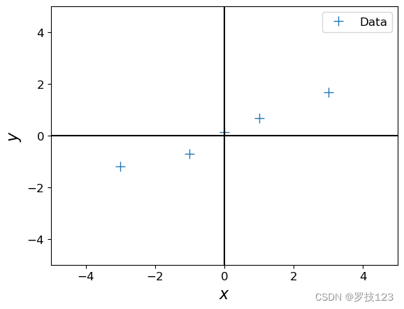
We will start with a simple training set, that we define by ourselves.
1 | # Define training set |
1 | <matplotlib.legend.Legend at 0x1341c3bd0> |
Section 2: Least squares loss and Maximum likelihood
From our lectures, we know that the parameters β \boldsymbol\beta β found by optimizing following equation:
min β ∥ y − X β ∥ 2 = min β L LS ( β ) \underset{\boldsymbol\beta}{\text{min}} \| \boldsymbol y - \boldsymbol X \boldsymbol\beta \|^2 = \underset{\boldsymbol\beta}{\text{min}} \ \text{L}_{\text{LS}} (\boldsymbol\beta) βmin∥y−Xβ∥2=βmin LLS(β)
where L LS \text{L}_{\text{LS}} LLS is the (ordinary) least squares loss function. The solution is
β ∗ = ( X T X ) − 1 X T y ∈ R ( p + 1 ) , \boldsymbol\beta^{*} = (\boldsymbol X^T\boldsymbol X)^{-1}\boldsymbol X^T\boldsymbol y \ \in\mathbb{R}^{(p+1)}\,, β∗=(XTX)−1XTy ∈R(p+1),
where
X = [ x 1 , … , x N ] T ∈ R N × ( p + 1 ) , y = [ y 1 , … , y N ] T ∈ R N . \boldsymbol X = [\boldsymbol x_1, \ldots, \boldsymbol x_N]^T\in\mathbb{R}^{N\times (p+1)}\,,\quad \boldsymbol y = [y_1, \ldots, y_N]^T \in\mathbb{R}^N\,. X=[x1,…,xN]T∈RN×(p+1),y=[y1,…,yN]T∈RN.
The same estimate of β \boldsymbol\beta β we can be obtained by maximum liklihood estimation which gives statistical interpretation of linear regression. In maximum likelihood estimation, we can find the parameters β M L \boldsymbol\beta^{\mathrm{ML}} βML that maximize the likelihood
p ( y ∣ X , β ) = ∏ n = 1 N p ( y n ∣ x n , β ) . p(\boldsymbol y | \boldsymbol X, \boldsymbol\beta) = \prod_{n=1}^N p(y_n | \boldsymbol x_n, \boldsymbol\beta)\,. p(y∣X,β)=n=1∏Np(yn∣xn,β).
From the lecture we know that the maximum likelihood estimator is given by
β ML = ( X T X ) − 1 X T y . \boldsymbol\beta^{\text{ML}} = (\boldsymbol X^T\boldsymbol X)^{-1}\boldsymbol X^T\boldsymbol y \, . βML=(XTX)−1XTy.
Let us compute the maximum likelihood estimate for the given training set.
1 | ## EDIT THIS FUNCTION |
1 | print(X.T @ X) |
1 | [[20]] |
1 | print(np.dot(X.T, X)) |
1 | [[20]] |
1 | #np.linalg.solve(a, b) -> gives a^(-1)b |
1 | # get maximum likelihood estimate |
Now, make a prediction using the maximum likelihood estimate that we just found.
1 | ## EDIT THIS FUNCTION |
1 | beta_ml |
1 | array([[0.499]]) |
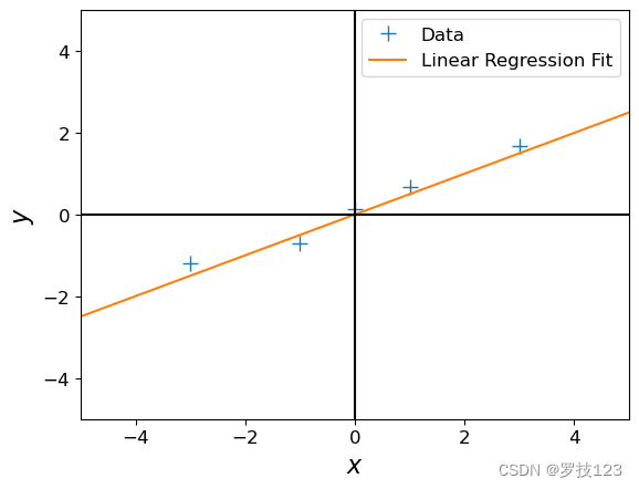
Let’s see whether we got something useful:
1 | # define a test set |
1 | <matplotlib.legend.Legend at 0x134801050> |
Questions
- Does the solution above look reasonable?
- Play around with different values of β \beta β. How do the corresponding functions change?
- Modify the training targets Y \mathcal Y Y and re-run your computation. What changes?
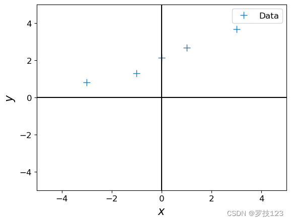
Let us now look at a different training set, where we add 2.0 to every y y y-value, and compute the maximum likelihood estimate.
1 | ynew = y + 2.0 |
1 | <matplotlib.legend.Legend at 0x1348b8710> |
1 | # get maximum likelihood estimate |
1 | [[0.499]] |
Question:
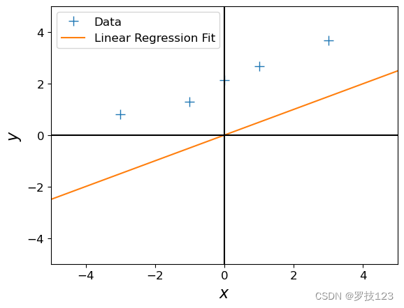
- This maximum likelihood estimate doesn’t look too good: The orange line is too far away from the observations although we just shifted them by 2. Why is this the case?
- How can we fix this problem?
Let us now define a linear regression model that is slightly more flexible:
y = β 0 + x T β 1 + ϵ , ϵ ∼ N ( 0 , σ 2 ) y = \beta_0 + \boldsymbol x^T \boldsymbol\beta_1 + \epsilon\,,\quad \epsilon\sim\mathcal N(0,\sigma^2) y=β0+xTβ1+ϵ,ϵ∼N(0,σ2)
Here, we added an offset (also called bias or intercept) parameter β 0 \beta_0 β0 to our original model.
Question:
- What is the effect of this bias parameter, i.e., what additional flexibility does it offer?
If we now define the inputs to be the augmented vector x aug = [ 1 x ] \boldsymbol x_{\text{aug}} = \begin{bmatrix}1\\\boldsymbol x\end{bmatrix} xaug=[1x], we can write the new linear regression model as
y = x aug T β aug + ϵ , β aug = [ β 0 β 1 ] . y = \boldsymbol x_{\text{aug}}^T\boldsymbol\beta_{\text{aug}} + \epsilon\,,\quad \boldsymbol\beta_{\text{aug}} = \begin{bmatrix} \beta_0\\ \boldsymbol\beta_1 \end{bmatrix}\,. y=xaugTβaug+ϵ,βaug=[β0β1].
1 | N, D = X.shape |
Let us now compute the maximum likelihood estimator for this setting.
Hint: If possible, re-use code that you have already written.
1 | ## EDIT THIS FUNCTION |
1 | beta_aug_ml = max_lik_estimate_aug(X_aug, ynew) |
1 | beta_aug_ml # offset + slope |
1 | array([[2.116], |
Now, we can make predictions again:
1 | # define a test set (we also need to augment the test inputs with ones) |
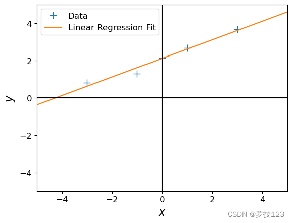
It seems this has solved our problem!
Question:
- Play around with the first parameter of β aug \boldsymbol\beta_{\text{aug}} βaug and see how the fit of the function changes.
- Play around with the second parameter of β aug \boldsymbol\beta_{\text{aug}} βaug and see how the fit of the function changes.
Section 3: Ridge regression
From our lectures, we know that ridge regression is an extension of linear regression with least squares loss function, including a (usually small) positive penalty term λ \lambda λ:
min β ∥ y − X β ∥ 2 + λ ∥ β ∥ 2 = min β L ridge ( β ) \underset{\boldsymbol\beta}{\text{min}} \| \boldsymbol y - \boldsymbol X \boldsymbol\beta \|^2 + \lambda \| \boldsymbol\beta \|^2 = \underset{\boldsymbol\beta}{\text{min}} \ \text{L}_{\text{ridge}} (\boldsymbol\beta) βmin∥y−Xβ∥2+λ∥β∥2=βmin Lridge(β)
where L ridge \text{L}_{\text{ridge}} Lridge is the ridge loss function. The solution is
β ridge ∗ = ( X T X + λ I ) − 1 X T y . \boldsymbol\beta^{*}_{\text{ridge}} = (\boldsymbol X^T\boldsymbol X + \lambda I)^{-1}\boldsymbol X^T\boldsymbol y \, . βridge∗=(XTX+λI)−1XTy.
This time, we will define a very small training set of only two observations to demonstrate the advantages of ridge regression over least squares linear regression.
1 | X_train = np.array([0.5, 1]).reshape(-1,1) |
Let’s define function similar to the one for least squares, but taking one additional argument, our penalty term λ \lambda λ.
Hint: we apply the same augmentation as above with least squares, so the offset is accurately captured.
1 | ## EDIT THIS FUNCTION |
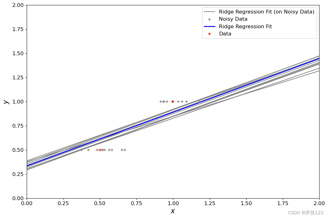
Now, we add a bit of Gaussian noise to our training set and apply ridge regression. We should do it a couple of times to be sure about the results (here 10 times).
1 | penalty_term = 0.1 |
1 | <matplotlib.legend.Legend at 0x134941050> |
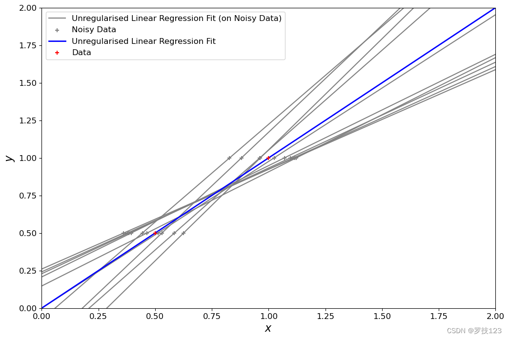
Let’s compare this to ordinary least squares:
1 | fig, ax = plt.subplots(figsize=(12, 8)) |
1 | <matplotlib.legend.Legend at 0x13427de50> |
Questions
- What differences between the two solutions above can you see?
- Optional:
- play around with different values of the penalty term λ \lambda λ. How do the corresponding functions change? Which values provide the most reasonable results?
- Can you replicate your results using
sklearn.linear_model.Ridge? - Based on sklearn’s documentation, can you see any differences in the algorithms that are implemented in sklearn?
Answers
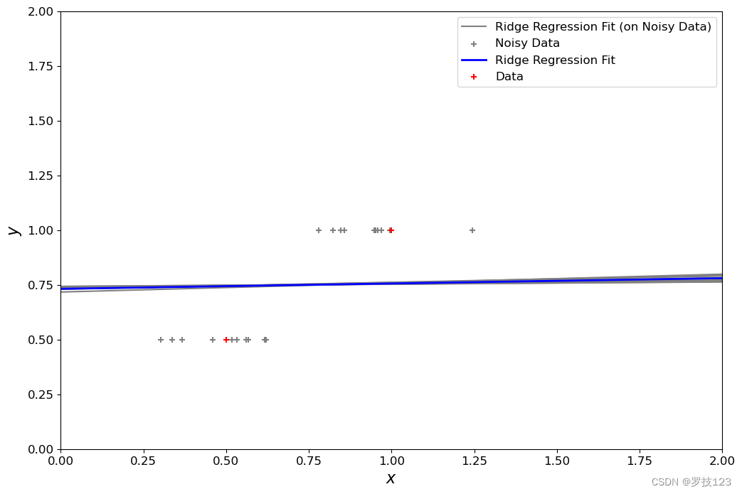
- For the standard regression, the performance on training points is very good, but can worsen on unseen test points, aka overfitting. Regularisation tends to constrain beta around more similar values, giving solutions with lower variance, but could become too close to zero with high lambda value.
1 | penalty_term = 5 |
1 | <matplotlib.legend.Legend at 0x134b74dd0> |
Take-Home Messages
- Models y = x T β + ϵ y = \boldsymbol x^T\boldsymbol\beta + \epsilon y=xTβ+ϵ with X = [ x 1 , … , x N ] T \boldsymbol X = [\boldsymbol x_1, \ldots, \boldsymbol x_N]^T X=[x1,…,xN]T and X = [ 1 , x 1 , … , x N ] T \boldsymbol X = [1,\boldsymbol x_1, \ldots, \boldsymbol x_N]^T X=[1,x1,…,xN]T are different in terms of flexibility
- A penalised regression with penalty term λ = 0 \lambda = 0 λ=0 is equivalent to the ordinary least squares regression
- After fitting your models, check whether the plots look as expected
Section 4: LASSO regression
As opposed to the ridge regression which has a penalty term ∥ β ∥ 2 \| \boldsymbol\beta \|^2 ∥β∥2, LASSO regression introduces $ | \boldsymbol\beta |_1 $, (also known as L 1 L_1 L1 loss). L 1 L_1 L1 loss is often preferred if we are interested in sparse parameters, i.e. few non-zero parameters. This is generally regarded as a feature selection task, and in high-dimensional problems it helps interpret the learned parameters and their relevance.
However, no closed-form solution exists for LASSO regression as in the standard and ridge regression, so we can use the iterative gradient-descent algorithm.
In LASSO regression the aim is to minimize the following loss:
L LASSO ( β ) = 1 2 N ∣ ∣ y − X β ∣ ∣ 2 + λ ∣ ∣ β ∣ ∣ 1 L_\text{LASSO}(\boldsymbol{\beta}) = \frac{1}{2N}|| \boldsymbol{y} - \boldsymbol{X} \boldsymbol{\beta}||^2 + \lambda ||\boldsymbol{\beta}||_1 LLASSO(β)=2N1∣∣y−Xβ∣∣2+λ∣∣β∣∣1Where ∣ ∣ β ∣ ∣ 1 = ∑ i = 1 p ∣ β i ∣ ||\boldsymbol{\beta}||_1 = \sum_{i=1}^p |\beta_i| ∣∣β∣∣1=∑i=1p∣βi∣
The absolute function ∣ . ∣ |.| ∣.∣ adds nonsmoothness to the loss function, which can prevent the gradient-descent to converge properly to the optimal solution, and will keep bouncing around it instead. To solve this, we can use the Huber loss as an alternative to the absolute function. It combines the behaviour of L 1 L_1 L1 loss except around the zero.
A relaxed optimization can be made by replacing ∣ ∣ β ∣ ∣ 1 ||\boldsymbol{\beta}||_1 ∣∣β∣∣1 with the Huber Loss ∑ i = 1 p L c ( β i ) \sum_{i=1}^p L_c(\beta_i) ∑i=1pLc(βi), where L c ( β ) L_c(\beta) Lc(β) is defined as:
$L_c (\beta) =
\begin{cases}
\frac{1}{2}{\beta^2} & \text{for } |\beta| \le c, \
c (|\beta| - \frac{1}{2}c), & \text{otherwise.}
\end{cases}
$
The c c c parameter in Huber determines the range around zero with L 2 L_2 L2-like behaviour to ensure smoothness and, hence, better convergence.
The piecewise smooth function L c ( β ) L_c (\beta) Lc(β) has the gradient:
$\frac{dL_c (\beta)}{d\beta} =
\begin{cases}
\beta & \text{for } |\beta| \le c, \
c, \text{sgn}(\beta) , & \text{otherwise.}
\end{cases}
$
Now we can minimize the following relaxed function by gradient descent:
$
\begin{align} L_\text{LASSO-Huber}(\boldsymbol{\beta})
&= \frac{1}{2N}|| \boldsymbol{y} - \boldsymbol{X} \boldsymbol{\beta}||^2 + \lambda \sum_i^p L_c(\beta) \
&= \frac{1}{2N}(\boldsymbol{y} - \boldsymbol{X}\boldsymbol{\beta})^T(\boldsymbol{y} - \boldsymbol{X}\boldsymbol{\beta}) + \lambda \sum_i^p L_c(\beta) \
&= \frac{1}{2N}\left(\boldsymbol{y}^T\boldsymbol{y} - \boldsymbol{y}^T\boldsymbol{X}\boldsymbol{\beta} - \boldsymbol{\beta}T\boldsymbol{X}T \boldsymbol{y} + \boldsymbol{\beta}T\boldsymbol{X}T\boldsymbol{X}\boldsymbol{\beta}\right) + \lambda \sum_i^p L_c(\beta)
\end{align}
$
Which has the gradient
$
\begin{align} \nabla_\boldsymbol{\beta} L_\text{LASSO-Huber}
&= \frac{1}{N}\left(\boldsymbol{X}^T\boldsymbol{X}\boldsymbol{\beta} - \boldsymbol{X}^T\boldsymbol{y}\right) + \lambda \nabla_{\boldsymbol{\beta}}L_c(\boldsymbol{\beta})
\end{align}$
Optimization method:
- Initialize β \boldsymbol{\beta} β with zeros.
- Use Gradient-descent for tuning β \boldsymbol{\beta} β
Implementated in Python as:
1 | def huber(beta, c = 1e-6): |
1 | a = np.linspace(-1, 1, 1000) |
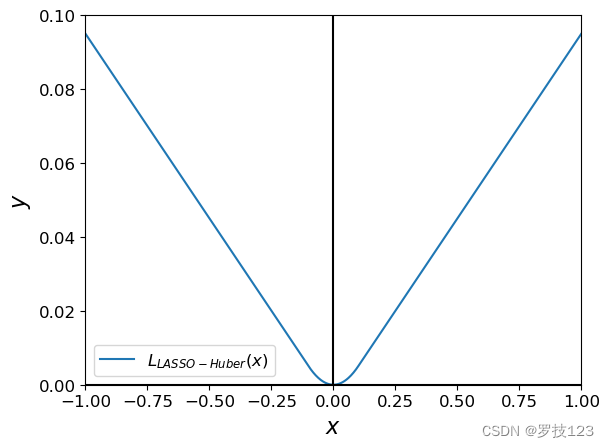
1 | a = np.linspace(-1, 1, 1000) |
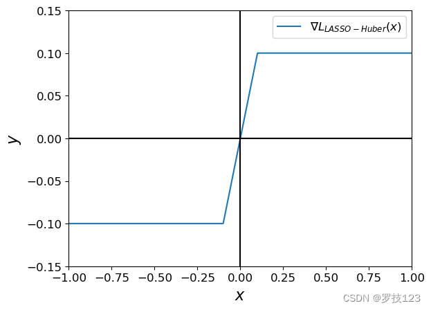
Try different c c c values and observe the difference
Optimization with gradient-descent
We next implement gradient-descent to solve the optimisation for the LASSO model.
1 | def minimize_ls_huber(X, y, lambd, n_iters = 10000, step_size=5e-5, c_huber=1e-4): |
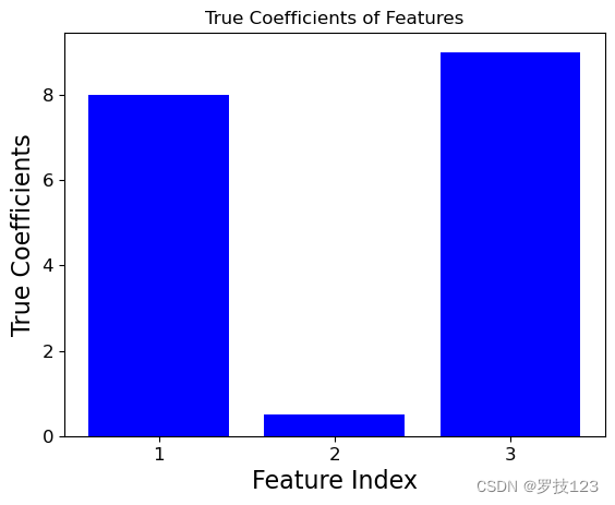
To study the feature selection capability of LASSO, we generate a 3 dimensional synthetic data set X X X where the second dimension does not contribute significantly to the target y y y.
1 | np.random.seed(42) |
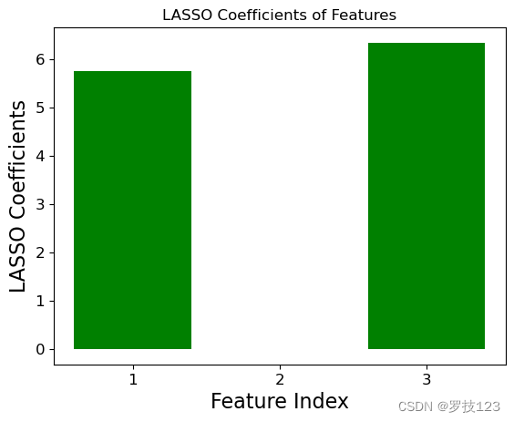
We can compare the ground truth coefficients used to create the synthetic data set to the optimal LASSO coefficients. We observe that the insignificant second feature has an optimal LASSO coefficent close to zero, and this illustrates that LASSO only selects the first and third feature as significant.
1 | # Add bias term |
1 | LASSO Regression Coefficients: |
1 | import matplotlib.pyplot as plt |
Questions
Try adding more insignicant variables and repeat the experiments. Do you still get the expected sparse solution? If not, what hyperparameters might need a re-tune?
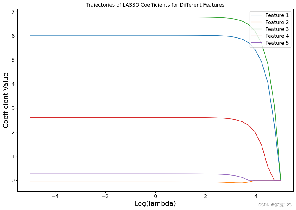
Can you observe a clear pattern in how coefficients change as the penalty term λ \lambda λ varies? Can you create a plot that shows the trajectory of each coefficient as λ \lambda λ changes?
Optional:
- Can you replicate your results using
sklearn.linear_model.Lasso? - Based on sklearn’s documentation, can you see any differences in the algorithms that are implemented in sklearn?
- Can you replicate your results using
Answers
We repeat the experiment on a five dimensional dataset X X X where the second and fifth dimensions contribute insignicantly to the target y y y.
1 | np.random.seed(0) |
We can now study the effect of the penality term λ \lambda λ on the LASSO coefficients.
1 | def lasso_coefficient_trajectories(lambdas, X_aug, y): |
1 | # define range for lambdas |
Plotting the trajectories of the LASSO coefficients for the 5 different features below shows us that the insiginifcant features 2 and 5 are always assigned LASSO coefficients close to zero. Only when the regularization is very strong, i.e., for large values of λ \lambda λ, all coefficients are pushed towards zero.
1 | # plot the trajectores of LASSO coefficients using log-scale |
 微信
微信 支付宝
支付宝