Docstring of split_samples function. It returns two tuples corresponding to the left and right splits.
Section 1: Decision Tree Classifier
Decision trees are a non-parametric supervised learning method used for classification and regression. The goal is to create a model that predicts the value of the label of unseen data by learning simple decision rules inferred from the data features.
You can understand it as using a set of if-then-else decision rules, e.g., if it snowed in London, then many Londoners would ski on Primrose Hill. Else, they would walk in Hyde Park. Generally speaking, the deeper the tree, i.e., the more if-then-else decisions are subsequently made in our model, the more complex the decision rules and the fitter the model. However, note that decision trees are prone to overfitting.
1
2
3
4
5
6
7
8
9
10
11
12
13
14
15
import numpy as np
import matplotlib.pyplot as plt

# Initial global configuration for matplotlib
SMALL_SIZE = 12
MEDIUM_SIZE = 16
BIGGER_SIZE = 20

plt.rc('font', size=SMALL_SIZE)          # controls default text sizes
plt.rc('axes', titlesize=SMALL_SIZE)     # fontsize of the axes title
plt.rc('axes', labelsize=MEDIUM_SIZE)    # fontsize of the x and y labels
plt.rc('xtick', labelsize=SMALL_SIZE)    # fontsize of the tick labels
plt.rc('ytick', labelsize=SMALL_SIZE)    # fontsize of the tick labels
plt.rc('legend', fontsize=SMALL_SIZE)    # legend fontsize
plt.rc('figure', titlesize=BIGGER_SIZE)  # fontsize of the figure title
In this notebook, we will use decision trees as a classification algorithm with the GINI-index, and work with the famous Iris data set. It contains four biological characteristics (features) of 150 samples that belong to three species (classes) of the family of Iris flowers (Iris setosa, Iris virginica and Iris versicolor). The data set provides 50 samples for each species.
1
2
3
4
5
# import packages
from collections import defaultdict
from sklearn.datasets import load_iris
import pandas as pd
import numpy as np
1
2
3
4
5
6
7
8
# load data
data = load_iris()
# print data to see how it is structured
#print(data)
X, y, column_names = data['data'], data['target'], data['feature_names']
# combining all information in one data frame
X_y = pd.DataFrame(X, columns=column_names)
X_y['label'] = y
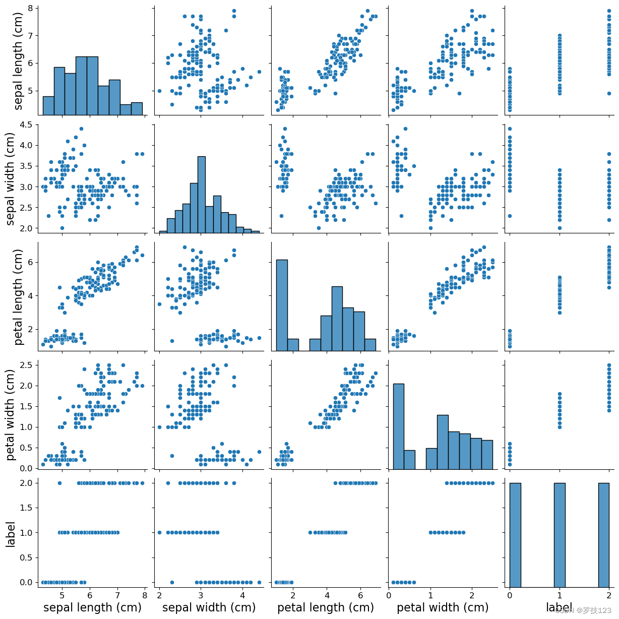
It is always a good idea to see whether the features are correlated. The python package seaborn has a nice one-line command called pairplot to explore this visually. It directly prints the feature names (sepal length, sepal width, petal length, petal width) and labels as axis titles. The pairplot plot below is used to visualize the distribution across samples of each descriptor and the correlation between descriptors (this helps identify collinear features).
1 2 3
import seaborn as sns
sns.pairplot(X_y);
1
We can observe some pairs of features are correlated with various degrees while others are not. We specifically observe that petal width and petal length are strongly correlated, while petal width is correlated sepal width with a lesser degree. We also observe that labels are balanced in this dataset.
As with any other supervised machine learning method, we create a train and test set to learn and evaluate our model, respectively.
# stacking data X and labels y into one matrix X_y_shuff = X_y.iloc[np.random.permutation(len(X_y))]
# we split train to test as 70:30 split_rate = 0.7 train, test = np.split(X_y_shuff, [int(split_rate*(X_y_shuff.shape[0]))])
# Separate the training features into X_train by extracting all columns except the last one, # which represent the labels, and vice versa for y_train. X_train = train[train.columns[:-1]] y_train = train[train.columns[-1]]
# Simlarly to test split. X_test = test[test.columns[:-1]] y_test = test[test.columns[-1]]
# We assume all examples have the same weight. training_weights = np.ones_like(y_train) / len(y_train)
# We need a dictionary indicating whether the column index maps to a # categorical feature or numerical # In this example, all features are numerical (categorical=False) columns_dict = {index: Falsefor index inrange(X_train.shape[1])}
We will build up our decision tree algorithm in the pythonic way how we have done it previously as well by calling functions we define first in functions we define later. For quick evaluations of your implementations, however, we have also included one-line commands after each cell to see whether your implementation results in errors.
Decision tree algorithm is a greedy algorithm that splits the data samples y \boldsymbol y y into lefty l \boldsymbol y_l yl and righty r \boldsymbol y_r yr samples, and the splitting is applied recursively on each side, resulting in a binary-tree like of splittings.
Samples can be split given two parameters: the feature index j j j and a value s s s.
If the feature is a continuous variable, the s s s is used as a threshold such that samples with feature value less than s s s are assigned to the left, and vice versa.
if the feature is a categorical variable, the s s s is used as a predicate such that samples with feature value equals to s s s are assigned to left, and vice versa.
To determine j j j and s s s at each split node, we may use GINI-index to search for j j j and s s s that minimizes the weighted sum of GINI-index of the left side samples and right side samples:
G I ( y ; j , s ) = p l × G I ( y l ) + p r × G I ( y r ) GI(\boldsymbol y; j, s) = p_l \times GI(\boldsymbol y_l) + p_r \times GI(\boldsymbol y_r) GI(y;j,s)=pl×GI(yl)+pr×GI(yr)
where p l p_l pl and p r p_r pr are, respectively, the cumulative weights of samples on the left and on the right, while G I ( y ) GI(\boldsymbol y) GI(y) is defined as:
GI ( y ) = 1 − ∑ i = 1 Q P ( y = c i ) 2 \text{GI}(\boldsymbol y) = 1 - \sum_{i=1}^Q \mathbb P (y = c_i)^2 GI(y)=1−i=1∑QP(y=ci)2
where c i c_i ci is the i-th class out of Q Q Q distinct classes, so P ( y = c i ) \mathbb P (y = c_i) P(y=ci) reads the weight of the class i i i in the current sample y \boldsymbol y y.
There are other alternatives to GINI-index like Information Gain but we will stick to GINI-index in this notebook.
It’s your turn to implement it in the next cell. We want to allow the code to consider samples with different weights, hence introduce an additional argument called sample_weights. The Iris data set we work with in this notebook has uniform sample weights, but other data sets you work with in the future could be different.
# EDIT THIS FUNCTION defgini_index(y, sample_weights): """ Calculate the GINI-index for labels. Arguments: y: vector of training labels, of shape (N,). sample_weights: weights for each samples, of shape (N,). Returns: (float): the GINI-index for y. """
# count different labels in y,and store in label_weights # initialize with zero for each distinct label. label_weights = {yi: 0for yi inset(y)} for yi, wi inzip(y, sample_weights): label_weights[yi] += wi
# The normalization constant total_weight = sum(label_weights.values()) # <-- SOLUTION
sum_p_squared = 0 for label, weight in label_weights.items(): sum_p_squared += (weight / total_weight)**2# <-- SOLUTION
Next, we define a function to split the data samples based on a feature (column) index and a value (recall how this value will be used whether the feature is categorical or numerical).
This has not much use yet, but we will call it in later functions, e.g., in the next cell in gini_split_value.
defsplit_samples(X, y, sample_weights, column, value, categorical): """ Return the split of data whose column-th feature: 1. equals value, in case `column` is categorical, or 2. less than value, in case `column` is not categorical (i.e. numerical) Arguments: X: training features, of shape (N, p). y: vector of training labels, of shape (N,). sample_weights: weights for each samples, of shape (N,). column: the column of the feature for splitting. value: splitting threshold the samples categorical: boolean value indicating whether column is a categorical variable or numerical. Returns: tuple(np.array, np.array, np.array): tuple of the left split data (X_l, y_l, w_l). tuple(np.array, np.array, np.array): tuple of the right split data (X_l, y_l, w_l) """
# Using the binary masks `left_mask`, we split X, y, and sample_weights. X_l, y_l, w_l = X[left_mask, :], y[left_mask], sample_weights[left_mask] # <- SOLUTION X_r, y_r, w_r = X[~left_mask, :], y[~left_mask], sample_weights[~left_mask] # <- SOLUTION
return (X_l, y_l, w_l), (X_r, y_r, w_r)
For a given feature index, we need to estimate the best value s s s to use as threshold (for numerical variables) or predicate (for categorical variables). We need to implement the function the searches for s s s that minimizes the GINI-index. Let’s do this in the following cell by calling our previously defined two functions split_samples and gini_index.
# EDIT THIS FUNCTION defgini_split_value(X, y, sample_weights, column, categorical): """ Calculate the GINI-index based on `column` with the split that minimizes the GINI-index. Arguments: X: training features, of shape (N, p). y: vector of training labels, of shape (N,). sample_weights: weights for each samples, of shape (N,). column: the column of the feature for calculating. 0 <= column < D categorical: boolean value indicating whether column is a categorical variable or numerical. Returns: (float, float): the resulted GINI-index and the corresponding value used in splitting. """
unique_vals = np.unique(X[:, column])
assertlen(unique_vals) > 1, f"There must be more than one distinct feature value. Given: {unique_vals}."
gini_index_val, threshold = np.inf, None
# split the values of i-th feature and calculate the cost for value in unique_vals: (X_l, y_l, w_l), (X_r, y_r, w_r) = split_samples(X, y, sample_weights, column, value, categorical) ## <-- SOLUTION
# if one of the two sides is empty, skip this split. iflen(y_l) == 0orlen(y_r) == 0: continue
## EDIT THIS FUNCTION defgini_split(X, y, sample_weights, columns_dict): """ Choose the best feature to split according to criterion. Args: X: training features, of shape (N, p). y: vector of training labels, of shape (N,). sample_weights: weights for each samples, of shape (N,). columns_dict: a dictionary mapping column indices to whether the column is categorical or numerical variable. Returns: (int, float): the best feature index and value used in splitting. If the feature index is None, then no valid split for the current Node. """
# Initialize `split_column` to None, so if None returned this means there is no valid split at the current node. min_gini_index = np.inf split_column = None split_val = np.nan
for column, categorical in columns_dict.items(): # skip column if samples are not seperable by that column. iflen(np.unique(X[:, column])) < 2: continue gini_index, current_split_val = gini_split_value(X, y, sample_weights, column, categorical) ## <-- SOLUTION
# evaluate which feature is best gini_split(X_train.to_numpy(), y_train.to_numpy(), training_weights, columns_dict)
1
(2, 3.3)
Now, we need a function that returns the label which appears the most in our label variable y.
1 2 3 4 5 6 7 8 9 10 11 12 13 14 15 16 17
defmajority_vote(y, sample_weights): """ Return the label which appears the most in y. Args: y: vector of training labels, of shape (N,). sample_weights: weights for each samples, of shape (N,). Returns: (int): the majority label """ majority_label = {yi: 0for yi inset(y)}
for yi, wi inzip(y, sample_weights): majority_label[yi] += wi
# EDIT THIS FUNCTION defbuild_tree(X, y, sample_weights, columns_dict, feature_names, depth, max_depth=10, min_samples_leaf=2): """Build the decision tree according to the data. Args: X: (np.array) training features, of shape (N, p). y: (np.array) vector of training labels, of shape (N,). sample_weights: weights for each samples, of shape (N,). columns_dict: a dictionary mapping column indices to whether the column is categorical or numerical variable. feature_names (list): record the name of features in X in the original dataset. depth (int): current depth for this node. Returns: (dict): a dict denoting the decision tree (binary-tree). Each node has seven attributes: 1. 'feature_name': The column name of the split. 2. 'feature_index': The column index of the split. 3. 'value': The value used for the split. 4. 'categorical': indicator for categorical/numerical variables. 5. 'majority_label': For leaf nodes, this stores the dominant label. Otherwise, it is None. 6. 'left': The left sub-tree with the same structure. 7. 'right' The right sub-tree with the same structure. Example: mytree = { 'feature_name': 'petal length (cm)', 'feature_index': 2, 'value': 3.0, 'categorical': False, 'majority_label': None, 'left': { 'feature_name': str, 'feature_index': int, 'value': float, 'categorical': bool, 'majority_label': None, 'left': {..etc.}, 'right': {..etc.} } 'right': { 'feature_name': str, 'feature_index': int, 'value': float, 'categorical': bool, 'majority_label': None, 'left': {..etc.}, 'right': {..etc.} } } """ # include a clause for the cases where (i) no feature, (ii) all labels are the same, (iii) depth exceed, or (iv) X is too small iflen(np.unique(y))==1or depth>=max_depth orlen(X)<=min_samples_leaf: return {'majority_label': majority_vote(y, sample_weights)}
split_index, split_val = gini_split(X, y, sample_weights, columns_dict) ## <-- SOLUTION
# If no valid split at this node, use majority vote. if split_index isNone: return {'majority_label': majority_vote(y, sample_weights)}
deftrain(X, y, columns_dict, sample_weights=None): """ Build the decision tree according to the training data. Args: X: (pd.Dataframe) training features, of shape (N, p). Each X[i] is a training sample. y: (pd.Series) vector of training labels, of shape (N,). y[i] is the label for X[i], and each y[i] is an integer in the range 0 <= y[i] <= C. Here C = 1. columns_dict: a dictionary mapping column indices to whether the column is categorical or numerical variable. sample_weights: weights for each samples, of shape (N,). """ if sample_weights isNone: # if the sample weights is not provided, we assume the samples have uniform weights sample_weights = np.ones(X.shape[0]) / X.shape[0] else: sample_weights = np.array(sample_weights) / np.sum(sample_weights)
feature_names = X.columns.tolist() X = X.to_numpy() y = y.to_numpy() return build_tree(X, y, sample_weights, columns_dict, feature_names, depth=1)
1
2
# fit the decision tree with training data tree = train(X_train, y_train, columns_dict)
Now, we want to use this fitted decision tree to make predictions for our test set X_test. To do so, we first define a function classify that takes each single data point x as an argument. We will write a wrapper function predict that calls this classify function. In the following implementation, we will traverse a given decision tree basen on the current feature vector that we have. Traversing tree-like objects in programming is straightforwardly implemented using recursion. If you are not familiar with recursion, check the following tutorial Python Recursion.
# EDIT THIS FUNCTION defclassify(tree, x): """ Classify a single sample with the fitted decision tree. Args: x: ((pd.Dataframe) a single sample features, of shape (D,). Returns: (int): predicted testing sample label. """ if tree['majority_label'] isnotNone: return tree['majority_label']
elif tree['categorical']: if x[tree['feature_index']] == tree['value']: # go to left branch return classify(tree['left'], x) else: # go to right branch return classify(tree['right'], x)
else:
if x[tree['feature_index']] < tree['value']: # <- SOLUTION # go to left branch return classify(tree['left'], x) # <- SOLUTION else: # go to right branch return classify(tree['right'], x) # <- SOLUTION
1 2 3 4 5 6 7 8 9 10 11 12
defpredict(tree, X): """ Predict classification results for X. Args: X: (pd.Dataframe) testing sample features, of shape (N, p). Returns: (np.array): predicted testing sample labels, of shape (N,). """ iflen(X.shape) == 1: return classify(tree, X) else: return np.array([classify(tree, x) for x in X])
To evaluate how well the tree can generalise to unseen data in X_test, we define a short function that computes the mean accuracy.
1 2 3 4
## EDIT THIS FUNCTION deftree_score(tree, X_test, y_test): y_pred = predict(tree, X_test) ## <-- SOLUTION return np.mean(y_pred==y_test)
Training accuracy: 0.9904761904761905 Test accuracy: 0.9111111111111111
Questions on Decision Trees:
What do the results above tell you? Has the decision tree you implemented overfitted to the training data?
If so, what can you change to counteract this problem?
Can you think of other information criteria than the GINI-index? If so, try implementing them and compare it to the decision tree with the GINI-index.
Recall ROC-curve (see Notebooks of Logistic Regression) that we used to compute the AUC as a more robust performance estimate, it required that each decision is associated with a probability (which can also be any kind of score representing the decision confidence). Suggest what can be used as score (or confidence) to be associated with each decision. Try to adapt for ROC-curve-compatible decisions and plot the ROC-curve indicating the AUC.
Can you provide another implementation of classify without using recursion?
training-samples used to mean the rows in X_train in other occasions, and we will use training-examples or training-instances instead to avoid confusion with
a random-sample, which means a selection of instances by chance from a group of instances.
It is now the time to build ensemble model from individual models for the first time in this course, applied to ensemble of decision trees.
One approach for ensemble methods is bootstrapping. In particular we can apply bootstrapping for multiple decision trees upon on levels:
Bootstrap on the training-instances: each model is trained on a random-sample (with replacement) from the training-instances. Eventually, as learned from lecture notes, decisions are aggregated across the models, hence the name bagging (Bootstrap Aggregate).
Note that for each decision tree we randomly-sample from training-instances with replacement and the size of each random-sample is the same size of the training-instances. This will basically allow some training-instances to be duplicated and other instances to be excluded.
Feature bagging: at each split, a subset of features are considered before searching for the best split column j j j and value s s s.
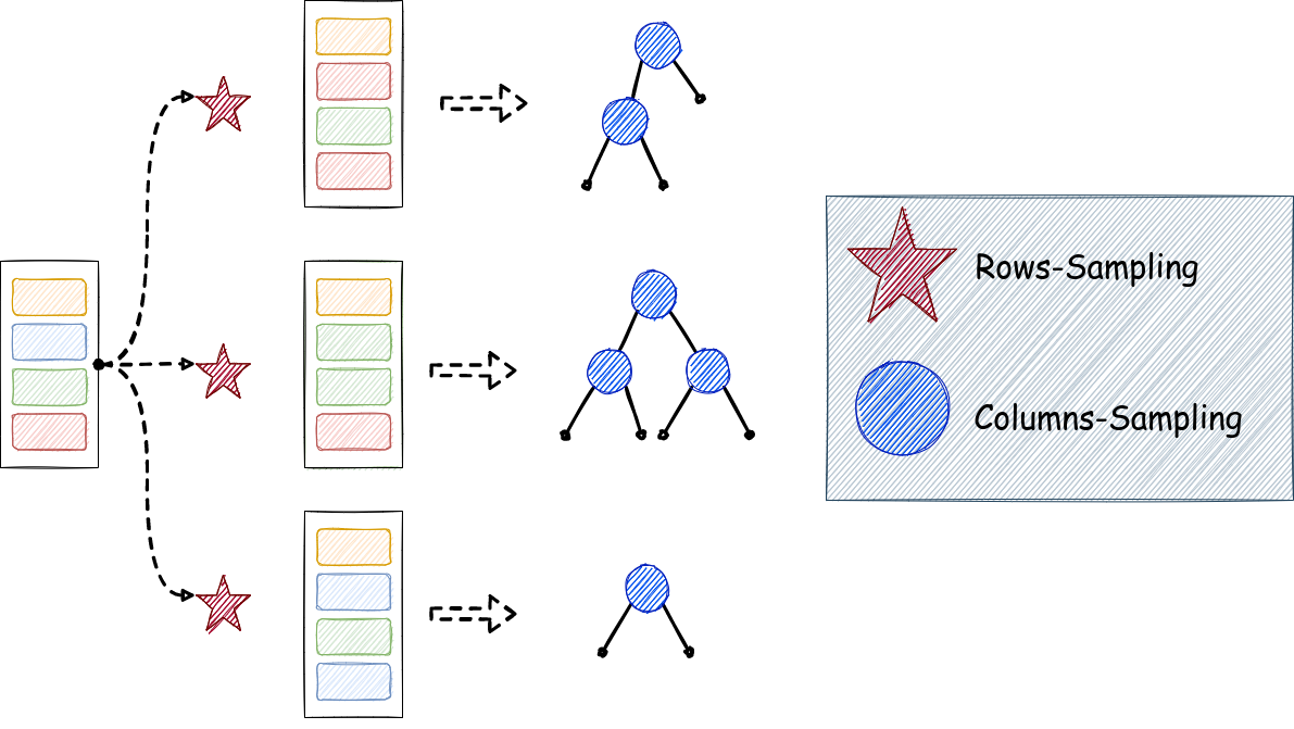
The image below illustrates random forest construction from individual decision trees. Notice the random-sampling that occurs at two levels:
At red-stars: bootstrapping (random-sampling with replacement) of training-instances.
At blue-circles: random-sampling without replacement of features at each split node.
This design will leave us two hyperparameters for random forest:
B B B: number of decision trees.
n_features: number of features (columns) sampled, without replacement, at each split before searching for the best split column j j j and value s s s. For classification task n_features is recommended to be the number of all columns divided by 3.
Add to these the decision trees hyperparameters like max_depth and min_leaf_sample.
The second layer of sampling, i.e. feature bagging, requires us to re-implement the gini_split function to subsample from the feature columns before searching for the best split.
Modify the following function that will be employed for random forest decision trees to find the best split column j j j (out from sampled n_features columns) and value s s s. Consider using the gini_split_value function that was already implemented for individual decision tree implementation.
Remember that we need to sample n_features from the column at each split, before we scan for the optimal splitting column. This will require us to make adapted versions of two of the decision tree functions:
gini_split: We need a new version gini_split_rf to add sampling step here before scanning for the optimal splitting column.
build_tree: because it depends on gini_split. We make another version build_tree_rf that calls gini_split_rf.
## EDIT THIS FUNCTION defgini_split_rf(n_features, X, y, sample_weights, columns_dict): """ Choose the best feature to split according to criterion. Args: n_features: number of sampled features. X: training features, of shape (N, p). y: vector of training labels, of shape (N,). sample_weights: weights for each samples, of shape (N,). columns_dict: a dictionary mapping column indices to whether the column is categorical or numerical variable. Returns: (float, int, float): the minimized gini-index, the best feature index and value used in splitting. """
# The added sampling step. columns = np.random.choice(list(columns_dict.keys()), n_features, replace=False) columns_dict = {c: columns_dict[c] for c in columns}
# Only scan through the sampled columns in `columns_dict`. for column, categorical in columns_dict.items(): # skip column if samples are not seperable by that column. iflen(np.unique(X[:, column])) < 2: continue
# search for the best splitting value for the given column. gini_index, val = gini_split_value(X, y, sample_weights, column, categorical) ## <-- SOLUTION if gini_index < min_gini_index: min_gini_index, split_column, split_val = gini_index, column, val
return min_gini_index, split_column, split_val
Since build_tree depends on gini_split, we need to slightly modify it to call gini_split_rf instead.
# EDIT THIS FUNCTION defbuild_tree_rf(n_features, X, y, sample_weights, columns_dict, feature_names, depth, max_depth=6, min_samples_leaf=5): """Build the decision tree according to the data. Args: X: (np.array) training features, of shape (N, p). y: (np.array) vector of training labels, of shape (N,). sample_weights: weights for each samples, of shape (N,). columns_dict: a dictionary mapping column indices to whether the column is categorical or numerical variable. feature_names (list): record the name of features in X in the original dataset. depth (int): current depth for this node. Returns: (dict): a dict denoting the decision tree (binary-tree). Each node has seven attributes: 1. 'feature_name': The column name of the split. 2. 'feature_index': The column index of the split. 3. 'value': The value used for the split. 4. 'categorical': indicator for categorical/numerical variables. 5. 'majority_label': For leaf nodes, this stores the dominant label. Otherwise, it is None. 6. 'left': The left sub-tree with the same structure. 7. 'right' The right sub-tree with the same structure. Example: mytree = { 'feature_name': 'petal length (cm)', 'feature_index': 2, 'value': 3.0, 'categorical': False, 'majority_label': None, 'left': { 'feature_name': str, 'feature_index': int, 'value': float, 'categorical': bool, 'majority_label': None, 'left': {..etc.}, 'right': {..etc.} } 'right': { 'feature_name': str, 'feature_index': int, 'value': float, 'categorical': bool, 'majority_label': None, 'left': {..etc.}, 'right': {..etc.} } } """ # include a clause for the cases where (i) all lables are the same, (ii) depth exceed (iii) X is too small iflen(np.unique(y)) == 1or depth>=max_depth orlen(X)<=min_samples_leaf: return {'majority_label': majority_vote(y, sample_weights)}
# EDIT THIS FUNCTION deftrain_rf(B, n_features, X, y, columns_dict, sample_weights=None): """ Build the decision tree according to the training data. Args: B: number of decision trees. X: (pd.Dataframe) training features, of shape (N, p). Each X[i] is a training sample. y: (pd.Series) vector of training labels, of shape (N,). y[i] is the label for X[i], and each y[i] is an integer in the range 0 <= y[i] <= C. Here C = 1. columns_dict: a dictionary mapping column indices to whether the column is categorical or numerical variable. sample_weights: weights for each samples, of shape (N,). """ if sample_weights isNone: # if the sample weights is not provided, we assume the samples have uniform weights sample_weights = np.ones(X.shape[0]) / X.shape[0] else: sample_weights = np.array(sample_weights) / np.sum(sample_weights)
feature_names = X.columns.tolist() X = X.to_numpy() y = y.to_numpy() N = X.shape[0] training_indices = np.arange(N) trees = []
for _ inrange(B): # Sample the training_indices (with replacement) sample = np.random.choice(training_indices, N, replace=True) # <- SOLUTION X_sample = X[sample, :] y_sample = y[sample] w_sample = sample_weights[sample] tree = build_tree_rf(n_features, X_sample, y_sample, w_sample, columns_dict, feature_names, depth=1) trees.append(tree)
defpredict_rf(rf, X): """ Predict classification results for X. Args: rf: A trained random forest through train_rf function. X: (pd.Dataframe) testing sample features, of shape (N, p). Returns: (np.array): predicted testing sample labels, of shape (N,). """
# EDIT THIS FUNCTION defaggregate(decisions): """ This function takes a list of predicted labels produced by a list of decision trees and returns the label with the majority of votes. """ count = defaultdict(int) for decision in decisions: count[decision] += 1 returnmax(count, key=count.get) # <- SOLUTION
iflen(X.shape) == 1: # if we have one sample return aggregate([classify(tree, X) for tree in rf]) else: # if we have multiple samples return np.array([aggregate([classify(tree, x) for tree in rf]) for x in X])
1 2 3 4
## EDIT THIS FUNCTION defrf_score(rf, X_test, y_test): y_pred = predict_rf(rf, X_test) ## <-- SOLUTION return np.mean(y_pred==y_test)
1 2 3 4 5
np.random.seed(0)
n_features = int(np.sqrt(X_train.shape[1]))
B = 30
# fit the random forest with training data
rf = train_rf(B, n_features, X_train, y_train, columns_dict)
Compare the test accuracy of a sole decision tree with random forest. What do you conclude?
How to make Random Forest decisions ROC-curve-compatible (i.e. decisions with confidence scores). Suggest what can be used as score (or confidence) to be associated with each decision. Try to plot a diagram with two ROC-curves:

 微信
微信 支付宝
支付宝