
这组文章整理自 2024 年的课程学习笔记,保留原练习、代码和图表。运行前请先看系列目录中的环境与数据说明。 查看系列目录。
Prerequisites
Outline
- Section 1: Dataset Preparation
- Section 2: Linear SVM Formulation
- Section 3: SVM Optimization using SGD
- Section 4: Model Evaluation via T-fold Cross Validation
Support Vector Machines (SVMs)
In this notebook, we will learn a linear and kernalised method of SVMs, which can be used for both regression and classification. To start with, we will focus on binary classification. We will use stochastic gradient descent (SGD) for the optimisation of the hinge loss.
We will work with the Breast Cancer Wisconsin (Diagnostic) Data Set, which you first need to download and then load in this notebook. If you faced difficulties downloading this data set from Kaggle, you should download the file directly from Blackboard. The data set contains various aspects of cell nuclei of breast screening images of patients with (malignant) and without (benign) breast cancer. Our goal is to build a classification model that can take these aspects of an unseen breast screening image, and classify it as either malignant or benign.
Section 1: Data Preparation
If you run this notebook locally on your machine, you will simply need to place the csv file in the same directory as this notebook.
If you run this notebook on Google Colab, you will need to use
from google.colab import files
upload = files.upload()
and then upload it from your local downloads directory.
1 | # necessary imports |
1 | #from google.colab import files |
1 | (569, 33) |
| id | diagnosis | radius_mean | texture_mean | perimeter_mean | area_mean | smoothness_mean | compactness_mean | concavity_mean | concave points_mean | … | texture_worst | perimeter_worst | area_worst | smoothness_worst | compactness_worst | concavity_worst | concave points_worst | symmetry_worst | fractal_dimension_worst | Unnamed: 32 | |
|---|---|---|---|---|---|---|---|---|---|---|---|---|---|---|---|---|---|---|---|---|---|
| 559 | 925291 | B | 11.51 | 23.93 | 74.52 | 403.5 | 0.09261 | 0.10210 | 0.11120 | 0.04105 | … | 37.16 | 82.28 | 474.2 | 0.12980 | 0.25170 | 0.3630 | 0.09653 | 0.2112 | 0.08732 | NaN |
| 560 | 925292 | B | 14.05 | 27.15 | 91.38 | 600.4 | 0.09929 | 0.11260 | 0.04462 | 0.04304 | … | 33.17 | 100.20 | 706.7 | 0.12410 | 0.22640 | 0.1326 | 0.10480 | 0.2250 | 0.08321 | NaN |
| 561 | 925311 | B | 11.20 | 29.37 | 70.67 | 386.0 | 0.07449 | 0.03558 | 0.00000 | 0.00000 | … | 38.30 | 75.19 | 439.6 | 0.09267 | 0.05494 | 0.0000 | 0.00000 | 0.1566 | 0.05905 | NaN |
| 562 | 925622 | M | 15.22 | 30.62 | 103.40 | 716.9 | 0.10480 | 0.20870 | 0.25500 | 0.09429 | … | 42.79 | 128.70 | 915.0 | 0.14170 | 0.79170 | 1.1700 | 0.23560 | 0.4089 | 0.14090 | NaN |
| 563 | 926125 | M | 20.92 | 25.09 | 143.00 | 1347.0 | 0.10990 | 0.22360 | 0.31740 | 0.14740 | … | 29.41 | 179.10 | 1819.0 | 0.14070 | 0.41860 | 0.6599 | 0.25420 | 0.2929 | 0.09873 | NaN |
| 564 | 926424 | M | 21.56 | 22.39 | 142.00 | 1479.0 | 0.11100 | 0.11590 | 0.24390 | 0.13890 | … | 26.40 | 166.10 | 2027.0 | 0.14100 | 0.21130 | 0.4107 | 0.22160 | 0.2060 | 0.07115 | NaN |
| 565 | 926682 | M | 20.13 | 28.25 | 131.20 | 1261.0 | 0.09780 | 0.10340 | 0.14400 | 0.09791 | … | 38.25 | 155.00 | 1731.0 | 0.11660 | 0.19220 | 0.3215 | 0.16280 | 0.2572 | 0.06637 | NaN |
| 566 | 926954 | M | 16.60 | 28.08 | 108.30 | 858.1 | 0.08455 | 0.10230 | 0.09251 | 0.05302 | … | 34.12 | 126.70 | 1124.0 | 0.11390 | 0.30940 | 0.3403 | 0.14180 | 0.2218 | 0.07820 | NaN |
| 567 | 927241 | M | 20.60 | 29.33 | 140.10 | 1265.0 | 0.11780 | 0.27700 | 0.35140 | 0.15200 | … | 39.42 | 184.60 | 1821.0 | 0.16500 | 0.86810 | 0.9387 | 0.26500 | 0.4087 | 0.12400 | NaN |
| 568 | 92751 | B | 7.76 | 24.54 | 47.92 | 181.0 | 0.05263 | 0.04362 | 0.00000 | 0.00000 | … | 30.37 | 59.16 | 268.6 | 0.08996 | 0.06444 | 0.0000 | 0.00000 | 0.2871 | 0.07039 | NaN |
10 rows × 33 columns
We can see that our data set has 569 samples and 33 columns. The column id can be taken as an index for our pandas dataframe and diagnosis is the label (either M: malignant or B: benign).
Let’s prepare the data set first of all by (i) cleaning it, (ii) separating label from features, and (iii) splitting it into train and test sets.
1 | # drop last column (extra column added by pd) |
| diagnosis | radius_mean | texture_mean | perimeter_mean | area_mean | smoothness_mean | compactness_mean | concavity_mean | concave points_mean | symmetry_mean | … | radius_worst | texture_worst | perimeter_worst | area_worst | smoothness_worst | compactness_worst | concavity_worst | concave points_worst | symmetry_worst | fractal_dimension_worst | |
|---|---|---|---|---|---|---|---|---|---|---|---|---|---|---|---|---|---|---|---|---|---|
| id | |||||||||||||||||||||
| 926424 | M | 21.56 | 22.39 | 142.00 | 1479.0 | 0.11100 | 0.11590 | 0.24390 | 0.13890 | 0.1726 | … | 25.450 | 26.40 | 166.10 | 2027.0 | 0.14100 | 0.21130 | 0.4107 | 0.2216 | 0.2060 | 0.07115 |
| 926682 | M | 20.13 | 28.25 | 131.20 | 1261.0 | 0.09780 | 0.10340 | 0.14400 | 0.09791 | 0.1752 | … | 23.690 | 38.25 | 155.00 | 1731.0 | 0.11660 | 0.19220 | 0.3215 | 0.1628 | 0.2572 | 0.06637 |
| 926954 | M | 16.60 | 28.08 | 108.30 | 858.1 | 0.08455 | 0.10230 | 0.09251 | 0.05302 | 0.1590 | … | 18.980 | 34.12 | 126.70 | 1124.0 | 0.11390 | 0.30940 | 0.3403 | 0.1418 | 0.2218 | 0.07820 |
| 927241 | M | 20.60 | 29.33 | 140.10 | 1265.0 | 0.11780 | 0.27700 | 0.35140 | 0.15200 | 0.2397 | … | 25.740 | 39.42 | 184.60 | 1821.0 | 0.16500 | 0.86810 | 0.9387 | 0.2650 | 0.4087 | 0.12400 |
| 92751 | B | 7.76 | 24.54 | 47.92 | 181.0 | 0.05263 | 0.04362 | 0.00000 | 0.00000 | 0.1587 | … | 9.456 | 30.37 | 59.16 | 268.6 | 0.08996 | 0.06444 | 0.0000 | 0.0000 | 0.2871 | 0.07039 |
5 rows × 31 columns
We do a bit more preparation by converting the categorical labels into 1 for M and -1 for B.
1 | # convert categorical labels to numbers |
1 | id |
| radius_mean | texture_mean | perimeter_mean | area_mean | smoothness_mean | compactness_mean | concavity_mean | concave points_mean | symmetry_mean | fractal_dimension_mean | … | radius_worst | texture_worst | perimeter_worst | area_worst | smoothness_worst | compactness_worst | concavity_worst | concave points_worst | symmetry_worst | fractal_dimension_worst | |
|---|---|---|---|---|---|---|---|---|---|---|---|---|---|---|---|---|---|---|---|---|---|
| id | |||||||||||||||||||||
| 926424 | 21.56 | 22.39 | 142.00 | 1479.0 | 0.11100 | 0.11590 | 0.24390 | 0.13890 | 0.1726 | 0.05623 | … | 25.450 | 26.40 | 166.10 | 2027.0 | 0.14100 | 0.21130 | 0.4107 | 0.2216 | 0.2060 | 0.07115 |
| 926682 | 20.13 | 28.25 | 131.20 | 1261.0 | 0.09780 | 0.10340 | 0.14400 | 0.09791 | 0.1752 | 0.05533 | … | 23.690 | 38.25 | 155.00 | 1731.0 | 0.11660 | 0.19220 | 0.3215 | 0.1628 | 0.2572 | 0.06637 |
| 926954 | 16.60 | 28.08 | 108.30 | 858.1 | 0.08455 | 0.10230 | 0.09251 | 0.05302 | 0.1590 | 0.05648 | … | 18.980 | 34.12 | 126.70 | 1124.0 | 0.11390 | 0.30940 | 0.3403 | 0.1418 | 0.2218 | 0.07820 |
| 927241 | 20.60 | 29.33 | 140.10 | 1265.0 | 0.11780 | 0.27700 | 0.35140 | 0.15200 | 0.2397 | 0.07016 | … | 25.740 | 39.42 | 184.60 | 1821.0 | 0.16500 | 0.86810 | 0.9387 | 0.2650 | 0.4087 | 0.12400 |
| 92751 | 7.76 | 24.54 | 47.92 | 181.0 | 0.05263 | 0.04362 | 0.00000 | 0.00000 | 0.1587 | 0.05884 | … | 9.456 | 30.37 | 59.16 | 268.6 | 0.08996 | 0.06444 | 0.0000 | 0.0000 | 0.2871 | 0.07039 |
5 rows × 30 columns
As with any data set that has features over different ranges, it’s required to standardise the data before.
1 | ## EDIT THIS FUNCTION |
1 | X_std = standardise(X) |
| radius_mean | texture_mean | perimeter_mean | area_mean | smoothness_mean | compactness_mean | concavity_mean | concave points_mean | symmetry_mean | fractal_dimension_mean | … | radius_worst | texture_worst | perimeter_worst | area_worst | smoothness_worst | compactness_worst | concavity_worst | concave points_worst | symmetry_worst | fractal_dimension_worst | |
|---|---|---|---|---|---|---|---|---|---|---|---|---|---|---|---|---|---|---|---|---|---|
| id | |||||||||||||||||||||
| 926424 | 2.110995 | 0.721473 | 2.060786 | 2.343856 | 1.041842 | 0.219060 | 1.947285 | 2.320965 | -0.312589 | -0.931027 | … | 1.901185 | 0.117700 | 1.752563 | 2.015301 | 0.378365 | -0.273318 | 0.664512 | 1.629151 | -1.360158 | -0.709091 |
| 926682 | 1.704854 | 2.085134 | 1.615931 | 1.723842 | 0.102458 | -0.017833 | 0.693043 | 1.263669 | -0.217664 | -1.058611 | … | 1.536720 | 2.047399 | 1.421940 | 1.494959 | -0.691230 | -0.394820 | 0.236573 | 0.733827 | -0.531855 | -0.973978 |
| 926954 | 0.702284 | 2.045574 | 0.672676 | 0.577953 | -0.840484 | -0.038680 | 0.046588 | 0.105777 | -0.809117 | -0.895587 | … | 0.561361 | 1.374854 | 0.579001 | 0.427906 | -0.809587 | 0.350735 | 0.326767 | 0.414069 | -1.104549 | -0.318409 |
| 927241 | 1.838341 | 2.336457 | 1.982524 | 1.735218 | 1.525767 | 3.272144 | 3.296944 | 2.658866 | 2.137194 | 1.043695 | … | 1.961239 | 2.237926 | 2.303601 | 1.653171 | 1.430427 | 3.904848 | 3.197605 | 2.289985 | 1.919083 | 2.219635 |
| 92751 | -1.808401 | 1.221792 | -1.814389 | -1.347789 | -3.112085 | -1.150752 | -1.114873 | -1.261820 | -0.820070 | -0.561032 | … | -1.410893 | 0.764190 | -1.432735 | -1.075813 | -1.859019 | -1.207552 | -1.305831 | -1.745063 | -0.048138 | -0.751207 |
5 rows × 30 columns
1 | # split into train and test set |
1 | /tmp/ipykernel_4930/2016496295.py:3: FutureWarning: Support for multi-dimensional indexing (e.g. `obj[:, None]`) is deprecated and will be removed in a future version. Convert to a numpy array before indexing instead. |
Section 2: Linear SVM Formulation
We start with defining the hinge loss as
L ( w ) = 1 2 ∥ w ∥ 2 + λ ∑ i = 1 n max ( 0 , 1 − y i ( x ( i ) ⋅ w + b ) ) . \mathcal L (\boldsymbol w) = \frac{1}{2} \| \boldsymbol w \|^2 + \lambda \sum_{i=1}^n \max \bigg( 0, 1-y_i (x^{(i)} \cdot \boldsymbol w + b) \bigg) \, . L(w)=21∥w∥2+λi=1∑nmax(0,1−yi(x(i)⋅w+b)).
where w \boldsymbol w w is the vector of weights, λ \lambda λ the regularisation parameter, and b b b the intercept which is included in our X as an additional column of 1 1 1’s.
1 | # EDIT THIS FUNCTION |
Section 3: SVM Optimization using SGD
One way to optimize the cost is by using stochastic gradient descent (SGD) algorithm. In order to use SGD, we need to implement a function for the cost gradients with respect to w \boldsymbol w w.
1 | # calculate gradient of cost |
Both of the two previous functions are then used in SGD to update the weights iteratively with a given learning rate α \alpha α. We also implement a stop criterion that ends the learning as soon as the cost function has not changed more than a manually determined percentage.
We know that the learning happens through updating the weights according to
w = w − α ∂ L ∂ w \boldsymbol w = \boldsymbol w - \alpha \frac{\partial \mathcal L}{\partial \boldsymbol w} w=w−α∂w∂L
where ∂ L ∂ w \frac{\partial \mathcal L}{\partial \boldsymbol w} ∂w∂L is the gradient of the hinge loss we have computed in the previous cell.
1 | # EDIT THIS FUNCTION |
Now, we can take these functions and train a linear SVM with our training data.
1 | # train the model |
1 | Iteration is: 1, Cost is: 4.839282882996163 |
We can plot the cost against the iteractions to check nothing went wrong
1 | plt.plot(iterations, costs) |
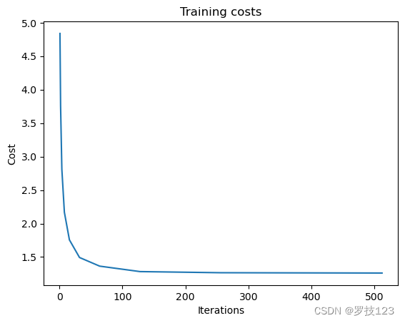
To evaluate the mean accuracy in both train and test set, we write a small function called score.
1 | ## EDIT THIS FUNCTION |
1 | Accuracy on training set: 0.9773869346733668 |
Questions:
- What are other evaluation metrics besides the accuracy? Implement them and assess the performance of our classification algorithm with them.
- What makes other evaluation metrics more appropriate given our unbalanced data set (we have more benign than malignant examples)?
- Try different learning rates, regularisation strengths and number of iterations independently. What can you observe? Can you achieve higher accuracies?
- What is your understanding why have we used the hinge loss with this data set of 31 features?
Section 4: Model Evaluation via T-fold Cross Validation
Now we repeat the same procedure as above but do not only have one train-test split, but multiple in a T-fold cross validation method.
1 | def cross_val_split(N, num_folds): |
1 | # evaluate |
1 | [array([ 84, 235, 170, 72, 64, 309, 108, 254, 222, 384, 325, 174, 106, |
1 | ## EDIT THIS FUNCTION |
1 | train_scores, val_scores = cross_val_evaluate(train, 5) |
1 | Fold 1 |
Finally, let’s compute the mean accuracy.
1 | print(np.mean(train_scores), np.mean(val_scores)) |
1 | 0.9893416927899686 0.9721518987341773 |
Subsection 4.1: Kernelised SVM
In the following, we implement a soft-margin kernelised SVM classifier with a non-linear kernel. Here, we use a Gaussian kernel:
k ( x , y ∣ σ ) = e − ∣ ∣ x − y ∣ ∣ 2 σ k(x,y|\sigma) = e^{-\frac{||x-y||^2}{\sigma}} k(x,y∣σ)=e−σ∣∣x−y∣∣2
1 | # First we need a function to calculate the kernel given the data # |
Having defined the kernel, we use this to compute the cost below.
1 | ## EDIT THIS FUNCTION |
As we have seen in the lecture notes, the kernel trick can be implemented in the primal-form problem by defining a new loss function:
L ( u , b ) = 1 2 u T K u + λ ∑ i = 1 N max { 0 , 1 − y ( i ) ( K ( i ) u + b ) } , L(\mathbf{u},b) = \frac{1}{2}\mathbf{u}^{\rm{T}}\mathbf{K} \mathbf{u} + \lambda \sum_{i=1}^N \max \Big\{0, 1-y^{(i)}(\mathbf{K}^{(i)}\mathbf{u} + b)\Big\}, L(u,b)=21uTKu+λi=1∑Nmax{0,1−y(i)(K(i)u+b)},where K \mathbf{K} K is the matrix containing the kernel functions, i.e.
K i j = k ( x ( i ) , x ( i ) ) \mathbf{K}_{ij} = k(\mathbf{x}^{(i)},\mathbf{x}^{(i)}) Kij=k(x(i),x(i)). To perform the optimisation, we simply modify the functions introduced above. Note that we will use X t r a i n X_{\mathrm{train}} Xtrain and X t e s t X_{\mathrm{test}} Xtest without the additional vector of ones. We had previously included this vector of ones to learn the intercept term b b b, but within the new formulation, one cannot readily employ this trick. How to include the intercept in kernalised SVM was a question in CW1 2023, and this year we make it an exercise in this notebook.
Following the steps above, we want to optimize the cost is by using SGD. First, we thus create a function that computes the gradients.
1 | ## EDIT THIS FUNCTION |
We can now use the functions above in SGD.
1 | ## EDIT THIS FUNCTION |
Finally, let’s compare some differnet values of σ.
1 | ## EDIT THIS FUNCTION |
1 | For sigma = 1 |
Questions:
- What do you observe varying sigma?
- How does the Gaussian Kernel SVM compare to the linear SVM?
Section 5: How to make a nice plot …
In your coursework, we ask you to produce some plots. Here, we outline how a “good” plot looks. For this purpose, let’s consider a specific example based on the data in this notebook. Thus, let’s plot the diagnosis (malignant or benign) in a scatter plot as a function of, say, the two first features (radius_mean and texture_mean). If we just plot the data using the standard settings, we don’t end up with a very good plot.
1 | plt.scatter(data_2.iloc[:, 1],data_2.iloc[:, 2],c=y); |
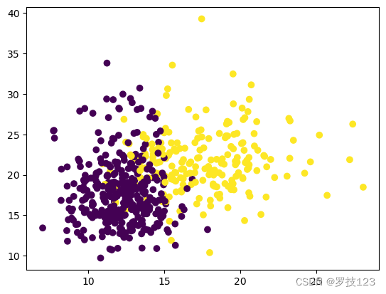
The problem is the following: As a rule of thumb, a plot should always be able to stand alone. In other words, it should be possible to understand the plot without reading the surrounding code or text and even (if possible) without reading the figure caption. The plot above can clearly not stand on its own. For starters, it doesn’t have any legend, nor does it have labels on the axes. Likewise, we should add a title. Other types of plots might have other options to add information. For instance, if we were dealing with a contour plot, we might want to include a colour bar or add labels to the contour lines.
1 | labels = ["Malignant", "Benign"] |
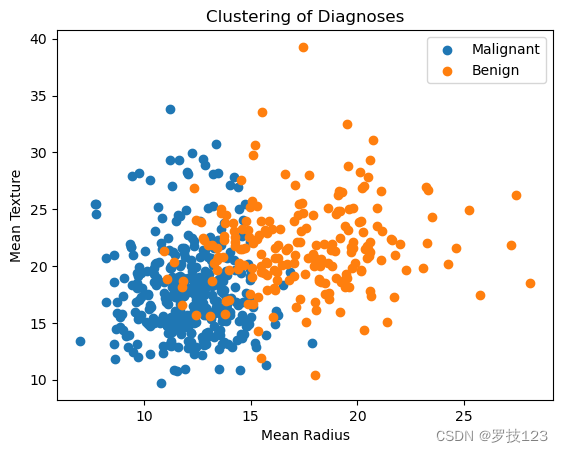
These small additions have improved the plot significantly. But it’s still not optimal. First of all, it’s rather small. To make it more readable, we should increase the figure size and change the font size of the different labels, titles, and ticks. Now, what is a suitable font size? As a rule of thumb, a plot should be easy to read when you print it. If you printed the notebook, the plot would be a bit on the small side since the text is smaller than the text in the cells; thus, if someone scrolls through your notebook, they would probably have to zoom in.
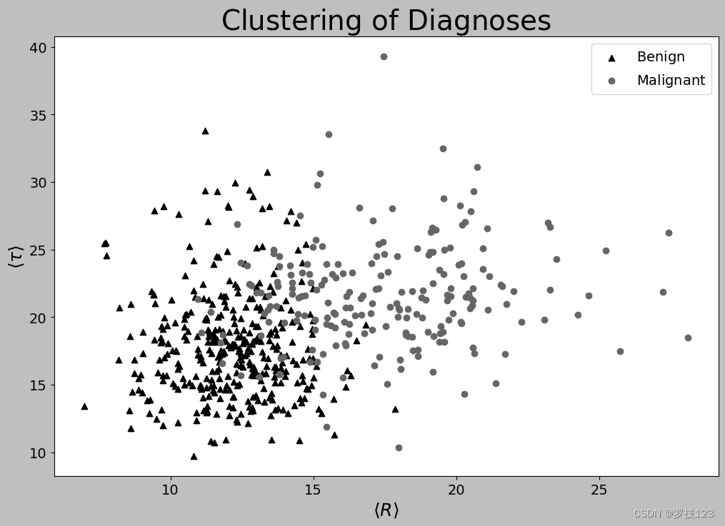
Secondly, we might want to reconsider the markers. Indeed, there is an addition to the rule stated above: A plot should be easy to read when you print it in grayscale. The idea is that you make the plot colourblind-friendly if you ensure that your plot is grayscale convertible. Thus, use colormaps that have this property. The default colormap of plt.scatter is actually grayscale convertible, leading to the choice of yellow and purple markers in the first plot in this section. While the notebook changed colours when creating the second plot, it chose colours that were “luckily” likewise grayscale convertible. If in doubt, you can, of course, use your own colour scheme, as shown below. Another way to make the plot more readable when printed in grayscale (and hence more readable in general) is to use different markers in addition to colours that are easily distinguishable. We, therefore, also change the markers themselves below. You can use the same trick when you make other plots. If you were to make, say, a line plot, you could consider, e.g., using different line styles (“-”,“:”,“–”).
1 | fig, ax = plt.subplots(figsize=(12,8)) # We make plot larger |
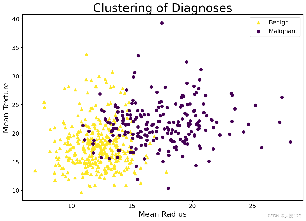
The plot above is what we would consider a “good” plot since it fulfils both the criteria sketched above: It can stand alone, and it’s easy to read. But what if we had decided to plot something different, such as the regularisation for the kernelised SVM, i.e. sigma? In that case, LaTeX commands would be useful for writing σ \sigma σ rather than “sigma”. Indeed, we can readily do so in Python by passing a raw string (r””) with a LaTeX command. So, for the sake of the example, let’s say that we have called the radius R and the texture τ \tau τ.
1 | # The plots in your report should be in colour. But just to show what we mean with grayscale convertable... |
 微信
微信 支付宝
支付宝